Indice dei Contenuti
- 1. Comprensione del Business e Domande
- 2. Caricamento e Panoramica dei Dati
- 3. Pulizia e Preparazione dei Dati
- 4. Integrazione dei Dati e Primi Insight di Business
- 5. Analisi di Prodotti e Categorie
- 6. Segmentazione Clienti – Analisi RFM
- 7. Analisi di Cohorts – Retention dei Clienti nel Tempo
- 8. Previsione Base – Predizione dei Ricavi Futuri con Prophet
- 9. Finalizzazione e Presentazione
Introduzione
Obiettivo del Progetto
Analisi orientata al business: vendite, comportamento del cliente, RFM, cohorts, CLV, previsione di base + raccomandazioni actionable.
Dataset
Dataset Pubblico Olist – ~100k ordini (Kaggle)
Tech Stack
- Python: pandas, seaborn, plotly, matplotlib, prophet
- Dashboard: Power BI
1. Comprensione del Business e Domande 
Domande chiave:
- Quali sono le categorie / prodotti top per ricavi?
- Retention e recurrenza dei clienti?
- Segmentazione RFM?
- Retention dei cohorts nel tempo?
- Performance di consegna per regione?
- Impatto dei metodi di pagamento?
- Opportunità di cross-sell?
- Previsione per le categorie top?
2. Caricamento e Panoramica dei Dati 
Questa sezione copre l'ingestione iniziale dei file CSV raw dal dataset Olist e fornisce una panoramica di alto livello sulla struttura, dimensione e contenuto di ciascuna tabella. L'obiettivo è confermare il caricamento riuscito, identificare le relazioni chiave tra le tabelle e individuare eventuali segnali immediati di qualità dei dati prima di procedere con la pulizia e l'analisi.
2.1. Caricamento dei Dati 
Carico le tabelle più rilevanti dal dataset Olist (orders, order_items, customers, payments, reviews) utilizzando pandas.
In questa fase vengono caricate solo le tabelle essenziali per mantenere basso l'uso della memoria e concentrarsi sulle entità principali necessarie per l'analisi di vendite, clienti e logistica.
# Imports
import pandas as pd
import matplotlib.pyplot as plt
import seaborn as sns
import plotly.express as px
import os
import plotly.graph_objects as go
from datetime import datetime
from prophet import Prophet
import plotly.io as pio

# set Plotly renderer so charts embed as interactive HTML instead of static images
pio.renderers.default = "notebook_connected"

# Settings for better visualizations
pd.set_option('display.max_columns', None)             # Show all columns
pd.set_option('display.max_rows', 100)                 # Show more rows
pd.set_option('display.float_format', '{:2f}'.format)  # Number formatting

sns.set_style("whitegrid")                             # Plot style
plt.rcParams['figure.figsize'] = (10, 6)               # Default figure size

print("Execution environment initialized successfully.")
print(f"• Pandas version: {pd.__version__}")
Execution environment initialized successfully.
• Pandas version: 2.3.3
# Base path to the data folder
data_path = './data/'

# Load key tables
orders = pd.read_csv(data_path + 'raw/olist_orders_dataset.csv')
order_items = pd.read_csv(data_path + 'raw/olist_order_items_dataset.csv')
customers = pd.read_csv(data_path + 'raw/olist_customers_dataset.csv')
payments = pd.read_csv(data_path + 'raw/olist_order_payments_dataset.csv')
reviews = pd.read_csv(data_path + 'raw/olist_order_reviews_dataset.csv')
2.2. Panoramica dei Dati e Controlli Iniziali 
Eseguo un'ispezione rapida di ciascuna tabella caricata per comprendere:
- Numero di righe e colonne
- Tipi di dati
- Presenza di valori mancanti
- Righe di esempio
Questo passo aiuta a mappare lo schema del dataset e decidere le priorità di pulizia successive.
# Quick look at each one
def quick_overview(df, name):
    print(f"\n=== {name.upper()} ===")
    print(f"Rows: {df.shape[0]:,}")
    print(f"Columns: {df.shape[1]}")
    print("\nData types and missing values:")
    print(df.info(verbose=False))
    print("\nFirst three rows:")
    display(df.head(3))  # display works better than print in Jupyter

quick_overview(orders, "Orders")
quick_overview(order_items, "Order Items")
quick_overview(customers, "Customers")
quick_overview(payments, "Payments")
quick_overview(reviews, "Reviews")
=== ORDERS ===
Rows: 99,441
Columns: 8

Data types and missing values:
<class 'pandas.core.frame.DataFrame'>
RangeIndex: 99441 entries, 0 to 99440
Columns: 8 entries, order_id to order_estimated_delivery_date
dtypes: object(8)
memory usage: 6.1+ MB
None

First three rows:
| order_id | customer_id | order_status | order_purchase_timestamp | order_approved_at | order_delivered_carrier_date | order_delivered_customer_date | order_estimated_delivery_date | |
|---|---|---|---|---|---|---|---|---|
| 0 | e481f51cbdc54678b7cc49136f2d6af7 | 9ef432eb6251297304e76186b10a928d | delivered | 2017-10-02 10:56:33 | 2017-10-02 11:07:15 | 2017-10-04 19:55:00 | 2017-10-10 21:25:13 | 2017-10-18 00:00:00 |
| 1 | 53cdb2fc8bc7dce0b6741e2150273451 | b0830fb4747a6c6d20dea0b8c802d7ef | delivered | 2018-07-24 20:41:37 | 2018-07-26 03:24:27 | 2018-07-26 14:31:00 | 2018-08-07 15:27:45 | 2018-08-13 00:00:00 |
| 2 | 47770eb9100c2d0c44946d9cf07ec65d | 41ce2a54c0b03bf3443c3d931a367089 | delivered | 2018-08-08 08:38:49 | 2018-08-08 08:55:23 | 2018-08-08 13:50:00 | 2018-08-17 18:06:29 | 2018-09-04 00:00:00 |
=== ORDER ITEMS ===
Rows: 112,650
Columns: 7

Data types and missing values:
<class 'pandas.core.frame.DataFrame'>
RangeIndex: 112650 entries, 0 to 112649
Columns: 7 entries, order_id to freight_value
dtypes: float64(2), int64(1), object(4)
memory usage: 6.0+ MB
None

First three rows:
| order_id | order_item_id | product_id | seller_id | shipping_limit_date | price | freight_value | |
|---|---|---|---|---|---|---|---|
| 0 | 00010242fe8c5a6d1ba2dd792cb16214 | 1 | 4244733e06e7ecb4970a6e2683c13e61 | 48436dade18ac8b2bce089ec2a041202 | 2017-09-19 09:45:35 | 58.900000 | 13.290000 |
| 1 | 00018f77f2f0320c557190d7a144bdd3 | 1 | e5f2d52b802189ee658865ca93d83a8f | dd7ddc04e1b6c2c614352b383efe2d36 | 2017-05-03 11:05:13 | 239.900000 | 19.930000 |
| 2 | 000229ec398224ef6ca0657da4fc703e | 1 | c777355d18b72b67abbeef9df44fd0fd | 5b51032eddd242adc84c38acab88f23d | 2018-01-18 14:48:30 | 199.000000 | 17.870000 |
=== CUSTOMERS ===
Rows: 99,441
Columns: 5

Data types and missing values:
<class 'pandas.core.frame.DataFrame'>
RangeIndex: 99441 entries, 0 to 99440
Columns: 5 entries, customer_id to customer_state
dtypes: int64(1), object(4)
memory usage: 3.8+ MB
None

First three rows:
| customer_id | customer_unique_id | customer_zip_code_prefix | customer_city | customer_state | |
|---|---|---|---|---|---|
| 0 | 06b8999e2fba1a1fbc88172c00ba8bc7 | 861eff4711a542e4b93843c6dd7febb0 | 14409 | franca | SP |
| 1 | 18955e83d337fd6b2def6b18a428ac77 | 290c77bc529b7ac935b93aa66c333dc3 | 9790 | sao bernardo do campo | SP |
| 2 | 4e7b3e00288586ebd08712fdd0374a03 | 060e732b5b29e8181a18229c7b0b2b5e | 1151 | sao paulo | SP |
=== PAYMENTS ===
Rows: 103,886
Columns: 5

Data types and missing values:
<class 'pandas.core.frame.DataFrame'>
RangeIndex: 103886 entries, 0 to 103885
Columns: 5 entries, order_id to payment_value
dtypes: float64(1), int64(2), object(2)
memory usage: 4.0+ MB
None

First three rows:
| order_id | payment_sequential | payment_type | payment_installments | payment_value | |
|---|---|---|---|---|---|
| 0 | b81ef226f3fe1789b1e8b2acac839d17 | 1 | credit_card | 8 | 99.330000 |
| 1 | a9810da82917af2d9aefd1278f1dcfa0 | 1 | credit_card | 1 | 24.390000 |
| 2 | 25e8ea4e93396b6fa0d3dd708e76c1bd | 1 | credit_card | 1 | 65.710000 |
=== REVIEWS ===
Rows: 99,224
Columns: 7

Data types and missing values:
<class 'pandas.core.frame.DataFrame'>
RangeIndex: 99224 entries, 0 to 99223
Columns: 7 entries, review_id to review_answer_timestamp
dtypes: int64(1), object(6)
memory usage: 5.3+ MB
None

First three rows:
| review_id | order_id | review_score | review_comment_title | review_comment_message | review_creation_date | review_answer_timestamp | |
|---|---|---|---|---|---|---|---|
| 0 | 7bc2406110b926393aa56f80a40eba40 | 73fc7af87114b39712e6da79b0a377eb | 4 | NaN | NaN | 2018-01-18 00:00:00 | 2018-01-18 21:46:59 |
| 1 | 80e641a11e56f04c1ad469d5645fdfde | a548910a1c6147796b98fdf73dbeba33 | 5 | NaN | NaN | 2018-03-10 00:00:00 | 2018-03-11 03:05:13 |
| 2 | 228ce5500dc1d8e020d8d1322874b6f0 | f9e4b658b201a9f2ecdecbb34bed034b | 5 | NaN | NaN | 2018-02-17 00:00:00 | 2018-02-18 14:36:24 |
3. Pulizia e Preparazione dei Dati 
3.1. Pulizia Iniziale dei Dati 
In questa fase eseguo controlli fondamentali di qualità dei dati: conversione delle colonne timestamp in formato datetime appropriato, verifica dell'unicità degli identificatori chiave (order_id, customer_id), e ispezione dei valori mancanti nelle colonne critiche. L'obiettivo è garantire che i dati raw siano affidabili e pronti per l'analisi senza introdurre errori nei calcoli o nei join.
Conversioni di tipo
Converto le stringhe timestamp in oggetti datetime per poter eseguire calcoli basati sul tempo (delta, raggruppamenti per mese, ecc.) in modo accurato.
# 3.1.1. Convert date columns to datetime

date_columns = [
    'order_purchase_timestamp',
    'order_approved_at',
    'order_delivered_carrier_date',
    'order_delivered_customer_date',
    'order_estimated_delivery_date'
]

for col in date_columns:
    orders[col] = pd.to_datetime(orders[col], errors='coerce')

print("Date columns converted:")
print(orders[date_columns].dtypes)
Date columns converted:
order_purchase_timestamp         datetime64[ns]
order_approved_at                datetime64[ns]
order_delivered_carrier_date     datetime64[ns]
order_delivered_customer_date    datetime64[ns]
order_estimated_delivery_date    datetime64[ns]
dtype: object
Controlli di Duplicati
Verifico che le chiavi primarie (order_id in orders, customer_id in customers) non abbiano duplicati, evitando conteggi gonfiati durante i merge o le aggregazioni.
# 3.1.2. Check duplicates in key tables

print("\nDuplicates:")
print("orders order_id duplicated:", orders['order_id'].duplicated().sum())
print("customers customer_id duplicated:", customers['customer_id'].duplicated().sum())
print("order_items (should be 0):", order_items.duplicated().sum())
Duplicates:
orders order_id duplicated: 0
customers customer_id duplicated: 0
order_items (should be 0): 0
Ispezione dei Valori Mancanti
Identifico e comprendo i pattern di dati mancanti, in particolare nei timestamp relativi alle consegne e nei commenti delle recensioni, per decidere strategie di gestione appropriate.
# 3.1.3. Missing values summary (focus on critical columns)

print("\nMissing values in orders:")
print(orders.isnull().sum()[orders.isnull().sum() > 0])

print("\nMissing values in reviews (expected high in comments):")
print(reviews.isnull().sum()[reviews.isnull().sum() > 0])
Missing values in orders:
order_approved_at                 160
order_delivered_carrier_date     1783
order_delivered_customer_date    2965
dtype: int64

Missing values in reviews (expected high in comments):
review_comment_title      87656
review_comment_message    58247
dtype: int64
3.2. Feature Engineering e Trasformazioni di Business 
Flag di Stato
Creo colonne booleane (is_delivered, is_approved) per filtrare facilmente ordini completati ed evitare problemi con NaN in metriche basate sul tempo.
# 3.2.1. Fill / handle missing timestamps in a business-friendly way

# Create flags (is_delivered, is_approved) for filtering later (e.g., only analyze delivered orders for delivery performance)
orders['is_delivered'] = orders['order_delivered_customer_date'].notna()
orders['is_approved'] = orders['order_approved_at'].notna()

print("Order status breakdown after cleaning:")
print(orders['order_status'].value_counts(normalize=True).round(3) * 100) # Use proportions (fractions that sum to 1), round to 3 d.p., and convert to %
Order status breakdown after cleaning:
order_status
delivered     97.000000
shipped        1.100000
canceled       0.600000
unavailable    0.600000
invoiced       0.300000
processing     0.300000
created        0.000000
approved       0.000000
Name: proportion, dtype: float64
Calcoli del Tempo di Consegna
Calcolo actual_delivery_time_days: i giorni di calendario reali dall'acquisto alla consegna al cliente — chiave per comprendere l'esperienza del cliente e la velocità logistica.
# 3.2.2. Calculate actual delivery time (from purchase to delivered) | how long the customer actually waited (purchase → delivered)
orders['actual_delivery_time_days'] = (
    orders['order_delivered_customer_date'] - orders['order_purchase_timestamp']
).dt.days
# 3.2.3. Calculate estimated vs actual delivery time difference | → positive = arrived late, negative = arrived early
orders['actual_minus_estimated_delivery_days'] = (
    orders['order_delivered_customer_date'] - orders['order_estimated_delivery_date']
).dt.days
Metriche di Ritardo e Performance
Calcolo actual_minus_estimated_delivery_days: quanto prima o dopo è arrivata l'ordine rispetto alla data promessa (negativo = anticipato, positivo = in ritardo) — essenziale per valutare l'accuratezza della promessa di consegna di Olist e il suo impatto sulla soddisfazione del cliente.
# Filter extreme outliers

reasonable_delivery = orders['actual_delivery_time_days'].between(0, 60)  # realistic range
print("\n% of orders with reasonable delivery time (0–60 days):", reasonable_delivery.mean().round(3) * 100)
% of orders with reasonable delivery time (0–60 days): 96.7
# Quick summary of new features

print("\nDelivery time stats (only delivered orders):")
delivered_orders = orders[orders['is_delivered']]             # Only consider delivered orders: Use mask 'orders['is_delivered']' to keep only rows where mask == True
print(delivered_orders[['actual_delivery_time_days', 'actual_minus_estimated_delivery_days']].describe())
Delivery time stats (only delivered orders):
       actual_delivery_time_days  actual_minus_estimated_delivery_days
count               96476.000000                          96476.000000
mean                   12.094086                            -11.876881
std                     9.551746                             10.183854
min                     0.000000                           -147.000000
25%                     6.000000                            -17.000000
50%                    10.000000                            -12.000000
75%                    15.000000                             -7.000000
max                   209.000000                            188.000000
4. Integrazione dei Dati e Primi Insight di Business 
4.1. Salvataggio dei Dati Puliti 
Salvo il DataFrame orders pulito e arricchito (con nuove feature) in una cartella di dati processati.
Questo segue le best practice: non sovrascrivere mai i dati raw e creare file intermedi riproducibili.
# 4.1 Saving Cleaned Data

# Create 'processed' subfolder if it doesn't exist
processed_dir = './data/processed/'
os.makedirs(processed_dir, exist_ok=True)

# Save the enriched orders table
orders.to_csv(processed_dir + 'cleaned_orders_with_features.csv', index=False)

print("Cleaned & enriched orders saved to:")
print(processed_dir + 'cleaned_orders_with_features.csv')
Cleaned & enriched orders saved to:
./data/processed/cleaned_orders_with_features.csv
4.2. Primo Merge – Creazione di una Tabella Base di Lavoro 
Combino le tabelle principali (orders + customers + payments) in un unico DataFrame master.
Questo fornisce una tabella unica con posizione del cliente, valore totale di pagamento e dettagli dell'ordine — ideale per analisi dei ricavi, segmentazione clienti e insight geografici.
# 4.2 First Merge – Creating a Base Working Table

# Step 1: Aggregate payments per order (some orders have multiple payments)
# I want total payment value per order_id
payments_total = payments.groupby('order_id')['payment_value'].sum().reset_index()
payments_total = payments_total.rename(columns={'payment_value': 'total_order_value'})

# Step 2: Merge orders + customers (get state and unique customer id)
base_df = orders.merge(
    customers[['customer_id', 'customer_unique_id', 'customer_state', 'customer_city']],
    on='customer_id',
    how='left'
)

# Step 3: Add total payment value
base_df = base_df.merge(
    payments_total,
    on='order_id',
    how='left'
)

# Quality check after merge
print("Shape before merges:", orders.shape)
print("Shape after merges:", base_df.shape)
print("\nMissing total_order_value after merge:", base_df['total_order_value'].isnull().sum())

# Show first few rows of our new base table
print("\nFirst 3 rows of base working table:")
display(base_df[['order_id', 'customer_unique_id', 'customer_state', 'order_status',
                 'actual_delivery_time_days', 'total_order_value']].head(3))
Shape before merges: (99441, 12)
Shape after merges: (99441, 16)

Missing total_order_value after merge: 1

First 3 rows of base working table:
| order_id | customer_unique_id | customer_state | order_status | actual_delivery_time_days | total_order_value | |
|---|---|---|---|---|---|---|
| 0 | e481f51cbdc54678b7cc49136f2d6af7 | 7c396fd4830fd04220f754e42b4e5bff | SP | delivered | 8.000000 | 38.710000 |
| 1 | 53cdb2fc8bc7dce0b6741e2150273451 | af07308b275d755c9edb36a90c618231 | BA | delivered | 13.000000 | 141.460000 |
| 2 | 47770eb9100c2d0c44946d9cf07ec65d | 3a653a41f6f9fc3d2a113cf8398680e8 | GO | delivered | 9.000000 | 179.120000 |
4.3. Primo Insight di Business: Ricavi e Performance di Consegna per Stato 
Aggrego la tabella base per calcolare il ricavo totale e il tempo medio di consegna per stato del cliente.
Questo fornisce una visione iniziale delle performance geografiche — identificando regioni ad alto valore e potenziali colli di bottiglia logistici.
# 4.3 First Business Insight: Revenue & Delivery Performance by State

# Filter only delivered orders (to make delivery metrics meaningful)
delivered_base = base_df[base_df['is_delivered']]

# Aggregate key metrics by state
state_summary = delivered_base.groupby('customer_state').agg(
    total_revenue=('total_order_value', 'sum'),
    avg_delivery_days=('actual_delivery_time_days', 'mean'),
    median_delivery_days=('actual_delivery_time_days', 'median'),
    order_count=('order_id', 'count'),
    avg_delay_days=('actual_minus_estimated_delivery_days', 'mean')
).reset_index()

# Format numbers for readability
state_summary['total_revenue'] = state_summary['total_revenue'].round(2)
state_summary['avg_delivery_days'] = state_summary['avg_delivery_days'].round(1)
state_summary['median_delivery_days'] = state_summary['median_delivery_days'].round(1)
state_summary['avg_delay_days'] = state_summary['avg_delay_days'].round(1)

# Add the average revenue per order for each state
state_summary['avg_revenue_per_order'] = (state_summary['total_revenue'] / state_summary['order_count']).round(2)

# Sort by total revenue descending
state_summary = state_summary.sort_values('total_revenue', ascending=False)

# Show top 10 states
print("Top 10 states by total revenue (delivered orders only):")
display(
    state_summary.head(10).style.format({
        'total_revenue': '{:,.2f}',
        'avg_delivery_days': '{:.1f}',
        'median_delivery_days': '{:.1f}',
        'order_count': '{:,}',
        'avg_delay_days': '{:.1f}',
        'avg_revenue_per_order': '{:,.2f}',
    })
)
Top 10 states by total revenue (delivered orders only):
| customer_state | total_revenue | avg_delivery_days | median_delivery_days | order_count | avg_delay_days | avg_revenue_per_order | |
|---|---|---|---|---|---|---|---|
| 25 | SP | 5,769,221.49 | 8.3 | 7.0 | 40,495 | -11.1 | 142.47 |
| 18 | RJ | 2,056,101.21 | 14.8 | 12.0 | 12,353 | -11.8 | 166.45 |
| 10 | MG | 1,819,321.70 | 11.5 | 10.0 | 11,355 | -13.2 | 160.22 |
| 22 | RS | 861,608.40 | 14.8 | 13.0 | 5,344 | -13.9 | 161.23 |
| 17 | PR | 781,919.55 | 11.5 | 10.0 | 4,923 | -13.3 | 158.83 |
| 23 | SC | 595,361.91 | 14.5 | 13.0 | 3,547 | -11.5 | 167.85 |
| 4 | BA | 591,270.60 | 18.9 | 16.0 | 3,256 | -10.8 | 181.59 |
| 6 | DF | 346,146.17 | 12.5 | 11.0 | 2,080 | -12.0 | 166.42 |
| 8 | GO | 334,294.22 | 15.2 | 13.0 | 1,957 | -12.2 | 170.82 |
| 7 | ES | 317,682.65 | 15.3 | 13.0 | 1,995 | -10.5 | 159.24 |
# Interactive bar chart with Plotly

fig = px.bar(
    state_summary.head(10),
    x='customer_state',
    y='total_revenue',
    color='avg_delivery_days',
    color_continuous_scale='RdYlGn_r',   # Red = late, Green = early
    title='Top 10 States by Revenue (color = avg actual delivery days)',
    labels={
        'customer_state': 'State',
        'total_revenue': 'Total Revenue (BRL)',
        'avg_delivery_days': 'Avg Delivery Time (days)'
    },
    hover_data=['order_count', 'median_delivery_days', 'avg_delay_days']
)

fig.update_layout(
    xaxis_title="State (UF)",
    yaxis_title="Total Revenue (BRL)",
    coloraxis_colorbar_title="Avg Delivery (days)"
)

fig.show()
Salvataggio del Riassunto per Stato
Esporto le metriche aggregate di performance per stato in un file processato per uso futuro (ad esempio, dashboarding in Power BI o visualizzazioni aggiuntive).
# 4.3.1 Saving State-Level Summary

# Reuse the same processed directory I created earlier
processed_dir = './data/processed/'
os.makedirs(processed_dir, exist_ok=True)

# Save the summary
state_summary.to_csv(
    processed_dir + 'state_performance_summary.csv',
    index=False
)

print("State summary saved successfully to:")
print(processed_dir + 'state_performance_summary.csv')
State summary saved successfully to:
./data/processed/state_performance_summary.csv
5. Analisi di Prodotti e Categorie 
5.1. Caricamento di Tabelle Aggiuntive 
Carico le tabelle relative ai prodotti per abilitare insight a livello di categoria.
products: attributi dei prodotti (categoria, dimensioni)product_category_name_translation: traduzione in inglese dei nomi delle categorie in portogheseorder_items: collega ordini ai prodotti (quantità, prezzo, spedizione) e già caricata precedentemente.
# 5.1 Loading Additional Tables

# Load the two new tables
products = pd.read_csv(data_path + 'raw/olist_products_dataset.csv')
category_translation = pd.read_csv(data_path + 'raw/product_category_name_translation.csv')

# Quick check
print("order_items shape:", order_items.shape)
print("products shape:", products.shape)
print("category_translation shape:", category_translation.shape)

# Preview both tables
quick_overview(products, "Products")
quick_overview(category_translation, "Category Translation")
order_items shape: (112650, 7)
products shape: (32951, 9)
category_translation shape: (71, 2)

=== PRODUCTS ===
Rows: 32,951
Columns: 9

Data types and missing values:
<class 'pandas.core.frame.DataFrame'>
RangeIndex: 32951 entries, 0 to 32950
Columns: 9 entries, product_id to product_width_cm
dtypes: float64(7), object(2)
memory usage: 2.3+ MB
None

First three rows:
| product_id | product_category_name | product_name_lenght | product_description_lenght | product_photos_qty | product_weight_g | product_length_cm | product_height_cm | product_width_cm | |
|---|---|---|---|---|---|---|---|---|---|
| 0 | 1e9e8ef04dbcff4541ed26657ea517e5 | perfumaria | 40.000000 | 287.000000 | 1.000000 | 225.000000 | 16.000000 | 10.000000 | 14.000000 |
| 1 | 3aa071139cb16b67ca9e5dea641aaa2f | artes | 44.000000 | 276.000000 | 1.000000 | 1000.000000 | 30.000000 | 18.000000 | 20.000000 |
| 2 | 96bd76ec8810374ed1b65e291975717f | esporte_lazer | 46.000000 | 250.000000 | 1.000000 | 154.000000 | 18.000000 | 9.000000 | 15.000000 |
=== CATEGORY TRANSLATION ===
Rows: 71
Columns: 2

Data types and missing values:
<class 'pandas.core.frame.DataFrame'>
RangeIndex: 71 entries, 0 to 70
Columns: 2 entries, product_category_name to product_category_name_english
dtypes: object(2)
memory usage: 1.2+ KB
None

First three rows:
| product_category_name | product_category_name_english | |
|---|---|---|
| 0 | beleza_saude | health_beauty |
| 1 | informatica_acessorios | computers_accessories |
| 2 | automotivo | auto |
5.2. Merge delle Informazioni sui Prodotti nella Tabella Base 
Unisco order_items con products e le traduzioni delle categorie, poi aggrego per ottenere metriche di performance per categoria (ricavi, conteggio ordini, prezzo medio, ecc.).
# 5.2 Merging Product Information

# Step 1: Translate category names (left join to keep all products)
products_en = products.merge(
    category_translation,
    on='product_category_name',
    how='left'
)

# Step 2: Merge order_items with products_en (add category, price, etc.)
items_with_category = order_items.merge(
    products_en[['product_id', 'product_category_name_english', 'product_weight_g']],
    on='product_id',
    how='left'
)

# Handle missing English category names
items_with_category['product_category_name_english'] = items_with_category['product_category_name_english'].fillna('uncategorized')

# Quick check for missing English names (should be very few)
print("Missing English category names:",
      items_with_category['product_category_name_english'].isnull().sum())

# Step 3: Aggregate by category (revenue, count, avg price, etc.)
category_performance = items_with_category.groupby('product_category_name_english').agg(
    total_revenue=('price', 'sum'),
    total_freight=('freight_value', 'sum'),
    order_items_count=('order_id', 'count'),
    unique_orders=('order_id', 'nunique'),
    avg_price=('price', 'mean'),
    avg_weight_g=('product_weight_g', 'mean')
).reset_index()

# Add revenue share %
total_revenue_all = category_performance['total_revenue'].sum()
category_performance['revenue_share_pct'] = (
    category_performance['total_revenue'] / total_revenue_all * 100
).round(2)

# Sort by revenue descending
category_performance = category_performance.sort_values('total_revenue', ascending=False)

# Show top 15 categories
print("\nTop 15 categories by total revenue:")
display(
    category_performance.head(15).style.format({
        'total_revenue': '{:,.2f}',
        'total_freight': '{:,.2f}',
        'avg_price': '{:,.2f}',
        'avg_weight_g': '{:.0f}',
        'revenue_share_pct': '{:.2f}%'
    })
)
Missing English category names: 0

Top 15 categories by total revenue:
| product_category_name_english | total_revenue | total_freight | order_items_count | unique_orders | avg_price | avg_weight_g | revenue_share_pct | |
|---|---|---|---|---|---|---|---|---|
| 43 | health_beauty | 1,258,681.34 | 182,566.73 | 9670 | 8836 | 130.16 | 1049 | 9.26% |
| 71 | watches_gifts | 1,205,005.68 | 100,535.93 | 5991 | 5624 | 201.14 | 581 | 8.87% |
| 7 | bed_bath_table | 1,036,988.68 | 204,693.04 | 11115 | 9417 | 93.30 | 2117 | 7.63% |
| 65 | sports_leisure | 988,048.97 | 168,607.51 | 8641 | 7720 | 114.34 | 1743 | 7.27% |
| 15 | computers_accessories | 911,954.32 | 147,318.08 | 7827 | 6689 | 116.51 | 903 | 6.71% |
| 39 | furniture_decor | 729,762.49 | 172,749.30 | 8334 | 6449 | 87.56 | 2653 | 5.37% |
| 20 | cool_stuff | 635,290.85 | 84,039.10 | 3796 | 3632 | 167.36 | 2549 | 4.67% |
| 49 | housewares | 632,248.66 | 146,149.11 | 6964 | 5884 | 90.79 | 3215 | 4.65% |
| 5 | auto | 592,720.11 | 92,664.21 | 4235 | 3897 | 139.96 | 2594 | 4.36% |
| 42 | garden_tools | 485,256.46 | 98,962.75 | 4347 | 3518 | 111.63 | 2824 | 3.57% |
| 69 | toys | 483,946.60 | 77,425.95 | 4117 | 3886 | 117.55 | 1857 | 3.56% |
| 6 | baby | 411,764.89 | 68,353.11 | 3065 | 2885 | 134.34 | 3273 | 3.03% |
| 59 | perfumery | 399,124.87 | 54,213.84 | 3419 | 3162 | 116.74 | 480 | 2.94% |
| 68 | telephony | 323,667.53 | 71,215.79 | 4545 | 4199 | 71.21 | 262 | 2.38% |
| 57 | office_furniture | 273,960.70 | 68,571.95 | 1691 | 1273 | 162.01 | 11390 | 2.02% |
5.3. Visualizzazione della Performance per Categoria e Insight 
Visualizzo le categorie top per ricavi e genero insight actionable su pricing, spedizione e opportunità.
# Top 10 categories for clean visualization
top_categories = category_performance.head(10)

# Bar chart: Revenue by category
fig_bar = px.bar(
    top_categories,
    x='product_category_name_english',
    y='total_revenue',
    color='avg_price',
    color_continuous_scale='YlOrRd',
    title='Top 10 Product Categories by Total Revenue',
    labels={
        'product_category_name_english': 'Category',
        'total_revenue': 'Total Revenue (BRL)',
        'avg_price': 'Average Unit Price (BRL)'
    },
    hover_data=['order_items_count', 'unique_orders', 'total_freight', 'revenue_share_pct']
)

fig_bar.update_layout(
    xaxis_title="Category",
    yaxis_title="Total Revenue (BRL)",
    xaxis_tickangle=-45,
    coloraxis_colorbar_title="Avg Price"
)

fig_bar.show()
# Pie chart: Revenue share (top 10 + others)
others_revenue = category_performance.iloc[10:]['total_revenue'].sum()

pie_data = pd.concat([
    top_categories[['product_category_name_english', 'total_revenue']],
    pd.DataFrame({'product_category_name_english': ['Others'], 'total_revenue': [others_revenue]})
])

fig_pie = px.pie(
    pie_data,
    values='total_revenue',
    names='product_category_name_english',
    title='Revenue Share - Top 10 Categories vs Others',
    hole=0.4  # donut style
)

fig_pie.show()
Osservazioni Chiave e Raccomandazioni Iniziali:
Salute e Bellezza guida con ~10 % del revenue totale: alto volume combinato con un prezzo medio solido → ideale per campagne di massa, promozioni per volume e sforzi di marketing ampi.
Letto, Bagno e Tavola e Arredamento e Decorazione mostrano costi di spedizione significativamente alti rispetto al prezzo → opportunità per rivedere il pricing (aumentare i margini) o negoziare tariffe logistiche migliori con i corrieri.
Orologi e Regali ha il ticket medio più alto (~201 BRL) → forte potenziale per upselling, bundle premium, raccomandazioni personalizzate e programmi fedeltà rivolti a clienti ad alto valore.
Le top 5 categorie rappresentano più del 40 % del revenue totale → alto rischio di concentrazione; considerare di diversificare promuovendo categorie emergenti o sottoperformanti.
1.627 articoli rimangono non categorizzati (~1–2 % del revenue) → vale la pena una revisione manuale per creare nuove categorie, migliorare la discoverability dei prodotti e potenziare gli algoritmi di raccomandazione.
5.4. Performance per Categoria e Stato 
Riunisco le informazioni sulle categorie con la tabella base dei clienti per analizzare quali categorie di prodotti performano meglio in ciascun stato brasiliano.
Questo aiuta a identificare preferenze regionali, opportunità localizzate e potenziali aggiustamenti logistici/pricing per regione.
# 5.4 Category Performance by State

# Step 1: Keep only delivered orders for meaningful metrics
delivered_base = base_df[base_df['is_delivered']].copy()

# Step 2: Add category info to delivered orders
# First, aggregate items by order_id (one row per order with main category)
# For simplicity, I take the category of the most expensive item per order (common approach)
order_main_category = (
    items_with_category.loc[
        items_with_category.groupby('order_id')['price'].idxmax()
    ]
    [['order_id', 'product_category_name_english']]
    .reset_index(drop=True)
)

# Merge main category into delivered_base
delivered_with_category = delivered_base.merge(
    order_main_category,
    on='order_id',
    how='left'
)

# Fill any missing categories (rare after previous fix)
delivered_with_category['product_category_name_english'] = delivered_with_category['product_category_name_english'].fillna('uncategorized')

# Step 3: Aggregate: revenue & order count per state + category
state_category_summary = delivered_with_category.groupby(
    ['customer_state', 'product_category_name_english']
).agg(
    total_revenue=('total_order_value', 'sum'),
    order_count=('order_id', 'nunique'),
    avg_ticket=('total_order_value', 'mean')
).reset_index()

# Add revenue share within each state
state_category_summary['state_total_revenue'] = state_category_summary.groupby('customer_state')['total_revenue'].transform('sum')
state_category_summary['revenue_share_in_state_pct'] = (
    state_category_summary['total_revenue'] / state_category_summary['state_total_revenue'] * 100
).round(2)

# Sort by state and then by revenue descending within state
state_category_summary = state_category_summary.sort_values(
    ['customer_state', 'total_revenue'], ascending=[True, False]
)

# Show top categories for the top 5 revenue states (SP, RJ, MG, RS, PR)
top_states = ['SP', 'RJ', 'MG', 'RS', 'PR']
for state in top_states:
    print(f"\nTop 10 categories in {state} by revenue:")
    display(
        state_category_summary[state_category_summary['customer_state'] == state]
        .head(10)
        .style.format({
            'total_revenue': '{:,.2f}',
            'avg_ticket': '{:,.2f}',
            'revenue_share_in_state_pct': '{:.2f}%',
            'state_total_revenue': '{:.2f}'
        })
    )
Top 10 categories in SP by revenue:
| customer_state | product_category_name_english | total_revenue | order_count | avg_ticket | state_total_revenue | revenue_share_in_state_pct | |
|---|---|---|---|---|---|---|---|
| 1272 | SP | bed_bath_table | 549,408.91 | 4307 | 127.56 | 5769221.49 | 9.52% |
| 1308 | SP | health_beauty | 509,859.18 | 3693 | 138.10 | 5769221.49 | 8.84% |
| 1335 | SP | watches_gifts | 449,135.06 | 2083 | 215.62 | 5769221.49 | 7.79% |
| 1329 | SP | sports_leisure | 427,734.06 | 3203 | 133.54 | 5769221.49 | 7.41% |
| 1280 | SP | computers_accessories | 386,706.97 | 2609 | 148.22 | 5769221.49 | 6.70% |
| 1304 | SP | furniture_decor | 331,287.25 | 2618 | 126.54 | 5769221.49 | 5.74% |
| 1314 | SP | housewares | 323,729.96 | 2693 | 120.21 | 5769221.49 | 5.61% |
| 1270 | SP | auto | 235,440.59 | 1579 | 149.11 | 5769221.49 | 4.08% |
| 1285 | SP | cool_stuff | 230,410.92 | 1279 | 180.15 | 5769221.49 | 3.99% |
| 1333 | SP | toys | 205,513.18 | 1568 | 131.07 | 5769221.49 | 3.56% |
Top 10 categories in RJ by revenue:
| customer_state | product_category_name_english | total_revenue | order_count | avg_ticket | state_total_revenue | revenue_share_in_state_pct | |
|---|---|---|---|---|---|---|---|
| 986 | RJ | watches_gifts | 188,485.58 | 784 | 240.42 | 2056101.21 | 9.17% |
| 924 | RJ | bed_bath_table | 175,594.31 | 1342 | 130.85 | 2056101.21 | 8.54% |
| 960 | RJ | health_beauty | 159,174.66 | 935 | 170.24 | 2056101.21 | 7.74% |
| 980 | RJ | sports_leisure | 140,578.56 | 889 | 158.13 | 2056101.21 | 6.84% |
| 932 | RJ | computers_accessories | 138,232.02 | 832 | 166.14 | 2056101.21 | 6.72% |
| 956 | RJ | furniture_decor | 118,425.00 | 809 | 146.38 | 2056101.21 | 5.76% |
| 966 | RJ | housewares | 93,000.20 | 709 | 131.17 | 2056101.21 | 4.52% |
| 937 | RJ | cool_stuff | 91,488.42 | 478 | 191.40 | 2056101.21 | 4.45% |
| 959 | RJ | garden_tools | 85,899.27 | 522 | 164.56 | 2056101.21 | 4.18% |
| 984 | RJ | toys | 83,263.44 | 539 | 154.48 | 2056101.21 | 4.05% |
Top 10 categories in MG by revenue:
| customer_state | product_category_name_english | total_revenue | order_count | avg_ticket | state_total_revenue | revenue_share_in_state_pct | |
|---|---|---|---|---|---|---|---|
| 514 | MG | health_beauty | 175,305.23 | 987 | 177.61 | 1819321.70 | 9.64% |
| 480 | MG | bed_bath_table | 155,527.65 | 1108 | 140.37 | 1819321.70 | 8.55% |
| 541 | MG | watches_gifts | 132,117.43 | 598 | 220.93 | 1819321.70 | 7.26% |
| 535 | MG | sports_leisure | 130,027.02 | 845 | 153.88 | 1819321.70 | 7.15% |
| 487 | MG | computers_accessories | 126,693.85 | 857 | 147.83 | 1819321.70 | 6.96% |
| 510 | MG | furniture_decor | 97,409.77 | 701 | 138.96 | 1819321.70 | 5.35% |
| 520 | MG | housewares | 92,826.66 | 676 | 137.32 | 1819321.70 | 5.10% |
| 478 | MG | auto | 82,521.85 | 458 | 180.18 | 1819321.70 | 4.54% |
| 492 | MG | cool_stuff | 79,890.81 | 422 | 189.31 | 1819321.70 | 4.39% |
| 513 | MG | garden_tools | 72,488.16 | 478 | 151.65 | 1819321.70 | 3.98% |
Top 10 categories in RS by revenue:
| customer_state | product_category_name_english | total_revenue | order_count | avg_ticket | state_total_revenue | revenue_share_in_state_pct | |
|---|---|---|---|---|---|---|---|
| 1098 | RS | bed_bath_table | 73,416.22 | 532 | 138.00 | 861608.40 | 8.52% |
| 1127 | RS | furniture_decor | 65,638.11 | 425 | 154.44 | 861608.40 | 7.62% |
| 1106 | RS | computers_accessories | 61,275.72 | 385 | 159.16 | 861608.40 | 7.11% |
| 1151 | RS | sports_leisure | 60,578.49 | 411 | 147.39 | 861608.40 | 7.03% |
| 1130 | RS | health_beauty | 59,453.00 | 388 | 153.23 | 861608.40 | 6.90% |
| 1157 | RS | watches_gifts | 51,874.17 | 222 | 233.67 | 861608.40 | 6.02% |
| 1111 | RS | cool_stuff | 49,747.79 | 251 | 198.20 | 861608.40 | 5.77% |
| 1136 | RS | housewares | 48,260.70 | 340 | 141.94 | 861608.40 | 5.60% |
| 1129 | RS | garden_tools | 38,871.63 | 219 | 177.50 | 861608.40 | 4.51% |
| 1155 | RS | toys | 33,347.80 | 200 | 166.74 | 861608.40 | 3.87% |
Top 10 categories in PR by revenue:
| customer_state | product_category_name_english | total_revenue | order_count | avg_ticket | state_total_revenue | revenue_share_in_state_pct | |
|---|---|---|---|---|---|---|---|
| 911 | PR | sports_leisure | 66,731.65 | 419 | 159.26 | 781919.55 | 8.53% |
| 917 | PR | watches_gifts | 62,263.22 | 265 | 234.96 | 781919.55 | 7.96% |
| 891 | PR | health_beauty | 61,366.50 | 375 | 163.64 | 781919.55 | 7.85% |
| 888 | PR | furniture_decor | 60,326.83 | 382 | 157.92 | 781919.55 | 7.72% |
| 859 | PR | bed_bath_table | 55,499.30 | 395 | 140.50 | 781919.55 | 7.10% |
| 866 | PR | computers_accessories | 50,583.03 | 333 | 151.90 | 781919.55 | 6.47% |
| 871 | PR | cool_stuff | 41,963.34 | 201 | 208.77 | 781919.55 | 5.37% |
| 897 | PR | housewares | 38,546.88 | 279 | 138.16 | 781919.55 | 4.93% |
| 857 | PR | auto | 32,421.59 | 202 | 160.50 | 781919.55 | 4.15% |
| 915 | PR | toys | 27,313.06 | 198 | 137.94 | 781919.55 | 3.49% |
5.5. Visualizzazione: Partecipazione dei Ricavi per Categoria e Stato 
Un heatmap mostra l'importanza relativa di ciascuna categoria all'interno degli stati principali, evidenziando preferenze regionali.
# 5.4.1 Visualization: Heatmap of Revenue Share by State and Category

# Filter to top 5 states and top 10 categories for readability
top_states = ['SP', 'RJ', 'MG', 'RS', 'PR']
top_cats = category_performance.head(10)['product_category_name_english'].tolist()

heatmap_df = state_category_summary[
    (state_category_summary['customer_state'].isin(top_states)) &
    (state_category_summary['product_category_name_english'].isin(top_cats))
]

# Pivot: states as rows, categories as columns, revenue share as values
pivot_table = heatmap_df.pivot(
    index='customer_state',      # rows
    columns='product_category_name_english',
    values='revenue_share_in_state_pct'
).fillna(0)

# Plot heatmap
plt.figure(figsize=(14, 6))

hm = sns.heatmap(
        pivot_table,
        annot=True,                # show numbers in cells
        fmt=".1f",
        annot_kws={"size": 12},    # font size of the numbers inside cells
        cmap="YlGnBu",
        linewidths=0.5,
        cbar_kws={'label': 'Revenue Share in State (%)'}
)

# Style the colorbar label
cbar = hm.collections[0].colorbar
cbar.set_label(
    'Revenue Share in State (%)',
    fontsize=16,               # ← adjust this number (16 is noticeably larger)
    fontweight='bold',
    labelpad=15
)
cbar.ax.tick_params(labelsize=12) # larger ticks on colorbar

plt.title('Revenue Share (%) – Top Categories in Top 5 States', fontsize=20, fontweight='bold', pad=25)
plt.xlabel('Category', fontsize=16, fontweight='bold', labelpad=10)
plt.ylabel('State (UF)', fontsize=16, fontweight='bold', labelpad=25)
plt.xticks(rotation=45, ha='right', fontsize=14)
plt.yticks(fontsize=14)
plt.tight_layout()
plt.show()

Insight Regionali per Categoria e Raccomandazioni:
São Paulo (SP): Dominato da letto_bagno_tavola (~9.5%), salute_bellezza (8.8%) e orologi_regali → mercato maturo con domanda diversificata; priorizzare bundle su articoli per la casa + bellezza e annunci mirati in queste categorie.
Rio de Janeiro (RJ) e Minas Gerais (MG): Maggiore quota relativa in decorazione_mobili e articoli_casa → preferenza regionale per articoli domestici; considerare promozioni di spedizione gratuita o pricing localizzato per compensare la sensibilità al costo di spedizione.
Stati del Sud (RS, PR): Più equilibrato verso sport_ricreazione, giocattoli e cose_cool → possibile influenza stagionale/culturale; esplorare campagne estive o promozioni focalizzate sui bambini.
Opportunità generale: Personalizzare raccomandazioni di prodotti e marketing per stato (es. focus su bellezza in SP, mobili in MG/RJ) → potenziale aumento di conversione e valore medio dell'ordine.
6. Segmentazione Clienti – Analisi RFM 
6.1. Calcolo RFM 
Calcolo le metriche classiche RFM per ciascun cliente unico:
- Recency: Giorni dall'ultimo acquisto (minore = più recente)
- Frequency: Numero di ordini effettuati
- Monetary: Ricavo totale generato dal cliente
Questo costituisce la base per segmentare i clienti in gruppi (es. VIP, a rischio, nuovi, persi) e derivare strategie di retention e upselling.
# 6.1 RFM Calculation

# Use only delivered orders for accurate purchase behavior
rfm_base = base_df[base_df['is_delivered']].copy()

# Current reference date (use the max purchase date + 1 day for realism)
reference_date = rfm_base['order_purchase_timestamp'].max() + pd.Timedelta(days=1)

# Aggregate per customer_unique_id
rfm = rfm_base.groupby('customer_unique_id').agg(
    recency=('order_purchase_timestamp', lambda x: (reference_date - x.max()).days), # Days since last purchase (lower number = more recent/active customer)
    frequency=('order_id', 'nunique'), # Number of distinct orders (higher = more loyal/repeat buyer)
    monetary=('total_order_value', 'sum') # Total BRL spent (higher = higher lifetime value)
).reset_index()

# Quick overview
print("RFM table shape:", rfm.shape)
print("\nRFM descriptive stats:")
print(rfm[['recency', 'frequency', 'monetary']].describe().round(2))

# Show top 10 customers by monetary value (VIP preview)
print("\nTop 10 customers by total spend:")
display(rfm.sort_values('monetary', ascending=False).head(10).style.format({
    'monetary': '{:,.2f}',
    'recency': '{:,}'
}))
RFM table shape: (93356, 4)

RFM descriptive stats:
           recency    frequency     monetary
count 93356.000000 93356.000000 93356.000000
mean    237.970000     1.030000   165.190000
std     152.620000     0.210000   226.320000
min       1.000000     1.000000     0.000000
25%     114.000000     1.000000    63.050000
50%     219.000000     1.000000   107.780000
75%     346.000000     1.000000   182.540000
max     714.000000    15.000000 13664.080000

Top 10 customers by total spend:
| customer_unique_id | recency | frequency | monetary | |
|---|---|---|---|---|
| 3724 | 0a0a92112bd4c708ca5fde585afaa872 | 334 | 1 | 13,664.08 |
| 79634 | da122df9eeddfedc1dc1f5349a1a690c | 515 | 2 | 7,571.63 |
| 43166 | 763c8b1c9c68a0229c42c9fc6f662b93 | 46 | 1 | 7,274.88 |
| 80461 | dc4802a71eae9be1dd28f5d788ceb526 | 563 | 1 | 6,929.31 |
| 25432 | 459bef486812aa25204be022145caa62 | 35 | 1 | 6,922.21 |
| 93079 | ff4159b92c40ebe40454e3e6a7c35ed6 | 462 | 1 | 6,726.66 |
| 23407 | 4007669dec559734d6f53e029e360987 | 279 | 1 | 6,081.54 |
| 87145 | eebb5dda148d3893cdaf5b5ca3040ccb | 498 | 1 | 4,764.34 |
| 26636 | 48e1ac109decbb87765a3eade6854098 | 69 | 1 | 4,681.78 |
| 73126 | c8460e4251689ba205045f3ea17884a1 | 22 | 4 | 4,655.91 |
6.2. Scoring RFM e Segmentazione Clienti 
Assegno punteggi (4 = migliore, 1 = peggiore) a Recency (minore = migliore), Frequency e Monetary.
- Recency e Monetary usano scoring basato sui quartili (
pd.qcut) - Frequency usa soglie personalizzate a causa dell'estrema skewness (97 % dei clienti acquista solo una volta)
Poi combino i punteggi in segmenti clienti actionable per strategie di retention, re-engagement e upselling.
# 6.2 RFM Scoring & Customer Segmentation

# 6.2.1. Create scores (quartiles)

# Recency: use qcut (works fine because recency is more spread out)
rfm['R_score'] = pd.qcut(rfm['recency'], q=4, labels=[4, 3, 2, 1])  # 4 = most recent

# Monetary: use qcut (also spread out)
rfm['M_score'] = pd.qcut(rfm['monetary'], q=4, labels=[1, 2, 3, 4])  # 4 = highest spend

# Frequency: custom thresholds because of heavy skew
def frequency_score(f):
    if f == 1:
        return 1
    elif f == 2:
        return 2
    elif 3 <= f <= 4:
        return 3
    else:  # f >= 5
        return 4

rfm['F_score'] = rfm['frequency'].apply(frequency_score)

# Combine scores
rfm['RFM_score'] = rfm['R_score'].astype(str) + rfm['F_score'].astype(str) + rfm['M_score'].astype(str)

print("Frequency score distribution:")
print(rfm['F_score'].value_counts(normalize=True).sort_index() * 100)

# 6.2.2. Define meaningful business segments
def get_segment(row):
    r = int(row['R_score'])
    f = int(row['F_score'])
    m = int(row['M_score'])

    if r >= 3 and f >= 3 and m >= 3:
        return 'Champions'                  # Best customers – recent, frequent, high value
    elif r >= 3 and f >= 2:
        return 'Loyal Customers'            # Recent & frequent/loyal
    elif r >= 4 and f == 1 and m >= 2:
        return 'Recent High-Value New'      # New but spent a lot recently
    elif r <= 2 and f >= 3:
        return 'At Risk'                    # Good past behavior, but inactive now
    elif r <= 2 and f <= 2 and m <= 2:
        return 'Lost / Hibernating'         # Inactive, low value
    else:
        return 'Other / Potential'          # Middle ground

rfm['segment'] = rfm.apply(get_segment, axis=1)

# 6.2.3. Summary table by segment
segment_summary = rfm.groupby('segment').agg(
    customer_count=('customer_unique_id', 'count'),
    avg_recency_days=('recency', 'mean'),
    avg_frequency=('frequency', 'mean'),
    avg_monetary=('monetary', 'mean'),
    total_revenue=('monetary', 'sum')
).reset_index()

# Add percentage columns
total_customers = segment_summary['customer_count'].sum()
total_revenue_all = segment_summary['total_revenue'].sum()

segment_summary['customer_share_pct'] = (segment_summary['customer_count'] / total_customers * 100).round(2)
segment_summary['revenue_share_pct'] = (segment_summary['total_revenue'] / total_revenue_all * 100).round(2)

# Sort by revenue descending
segment_summary = segment_summary.sort_values('total_revenue', ascending=False)

print("\nRFM Segments Summary:")
display(
    segment_summary.style.format({
        'avg_recency_days': '{:.1f}',
        'avg_frequency': '{:.2f}',
        'avg_monetary': '{:,.2f}',
        'total_revenue': '{:,.2f}',
        'customer_share_pct': '{:.2f}%',
        'revenue_share_pct': '{:.2f}%'
    })
)
Frequency score distribution:
F_score
1   96.999657
2    2.756116
3    0.223874
4    0.020352
Name: proportion, dtype: float64

RFM Segments Summary:
| segment | customer_count | avg_recency_days | avg_frequency | avg_monetary | total_revenue | customer_share_pct | revenue_share_pct | |
|---|---|---|---|---|---|---|---|---|
| 4 | Other / Potential | 51147 | 241.7 | 1.02 | 193.65 | 9,904,644.95 | 54.79% | 64.22% |
| 5 | Recent High-Value New | 16824 | 57.9 | 1.00 | 206.31 | 3,471,006.78 | 18.02% | 22.51% |
| 2 | Lost / Hibernating | 23750 | 365.1 | 1.01 | 63.98 | 1,519,629.32 | 25.44% | 9.85% |
| 3 | Loyal Customers | 1408 | 113.7 | 2.00 | 291.97 | 411,089.82 | 1.51% | 2.67% |
| 1 | Champions | 141 | 105.7 | 3.55 | 542.11 | 76,437.42 | 0.15% | 0.50% |
| 0 | At Risk | 86 | 362.9 | 3.15 | 453.76 | 39,023.14 | 0.09% | 0.25% |
6.3. Visualizzazione dei Segmenti RFM e Raccomandazioni Azionabili 
Visualizziamo la distribuzione di clienti e ricavi per segmento, poi deriviamo strategie concrete di business per ciascun gruppo (retention, re-engagement, upselling, aggiustamenti di pricing, ecc.).
# 6.3 RFM Segment Visualization

# 1. Bar chart: Customer count & Revenue share by segment
fig_bar = px.bar(
    segment_summary,
    x='segment',
    y=['customer_share_pct', 'revenue_share_pct'],
    barmode='group',
    title='<b>Customer Share vs Revenue Share by RFM Segment</b>',
    labels={
        'value': 'Percentage (%)',
        'variable': 'Metric',
        'segment': 'Customer Segment'
    },
    color_discrete_sequence=['#636EFA', '#EF553B']  # blue for customers, red for revenue
)

fig_bar.update_layout(
    title={'font': {'size': 18, 'color': 'black'}},
    xaxis_title="Segment",
    yaxis_title="Percentage (%)",
    legend_title="Metric",
    xaxis_tickangle=-45,
    height=500
)

fig_bar.show()
# 2. Pie chart: Revenue contribution by segment (focus on who drives the money)
fig_pie = px.pie(
    segment_summary,
    values='total_revenue',
    names='segment',
    title='Total Revenue Contribution by RFM Segment',
    hole=0.4,  # donut style
    color_discrete_sequence=px.colors.qualitative.Pastel
)

fig_pie.update_traces(textposition='inside', textinfo='percent+label')
fig_pie.update_layout(
    height=500,
    title={'font': {'size': 18, 'color': 'black'}}
)

fig_pie.show()
Raccomandazioni Azionabili per Segmento:
Altri / Potenziale (54.79 % clienti, 64.22 % ricavi)
Gruppo più grande, motore principale dei ricavi ma con performance media.
→ Concentrarsi sulla conversione verso segmenti superiori: email personalizzate con sconti sul prossimo acquisto, raccomandazioni cross-sell (es. bundle salute_bellezza con letto_bagno_tavola).
Nuovi ad Alto Valore Recenti (18.02 % clienti, 22.51 % ricavi)
Clienti nuovi con primo acquisto di alto valore — molto preziosi!
→ Nutrimento immediato post-acquisto: email di ringraziamento + invito al programma fedeltà, suggerire prodotti complementari (upsell bundle), spedizione gratuita sul secondo ordine per incoraggiare la ripetizione.
Persi / Inattivi (25.44 % clienti, 9.85 % ricavi)
Grande gruppo inattivo con valore passato.
→ Campagne di riattivazione: email win-back con offerte a tempo limitato (es. 20 % off + spedizione gratuita), sondaggio per capire la ragione del churn, annunci mirati su categorie ad alto margine che hanno comprato in passato.
Clienti Leali (1.51 % clienti, 2.67 % ricavi)
Gruppo piccolo ma che ripete acquisti.
→ Benefici VIP: accesso anticipato alle vendite, bundle esclusivi, sistema di punti fedeltà per aumentare frequenza e ticket medio.
Champions (0.15 % clienti, 0.50 % ricavi)
Gruppo élite — recenti, frequenti (per Olist), alto spend.
→ Trattamento premium: contatto personale, supporto dedicato, invito a beta/test di nuovi prodotti, programma referral con alte ricompense.
A Rischio (0.09 % clienti, 0.25 % ricavi)
Precedentemente buoni ma ora inattivi.
→ Riattivazione urgente: offerte personalizzate "ci manchi", sconti di alto valore a tempo limitato su categorie che hanno amato.
Opportunità Generale:
Con il 97 % di clienti one-time, il focus deve essere sull'aumento della frequenza in tutti i segmenti — bundle, abbonamenti (se possibile), programma fedeltà e consegne più rapide negli stati ad alto valore (SP/RJ) per migliorare soddisfazione e tasso di ripetizione.
6.4. Esportazione dei Risultati RFM 
Salvo la tabella RFM completa (con punteggi e segmenti) e il riassunto per segmento nella cartella dei dati processati.
Questi file possono essere usati direttamente in Power BI per dashboard interattivi o report aggiuntivi.
# 6.4 Exporting RFM Results

# Ensure processed folder exists
processed_dir = './data/processed/'
os.makedirs(processed_dir, exist_ok=True)

# 1. Save full RFM table (per customer)
rfm.to_csv(
    processed_dir + 'rfm_customers_with_segments.csv',
    index=False
)
print("Full RFM table saved to:")
print(processed_dir + 'rfm_customers_with_segments.csv')

# 2. Save segment summary (aggregated)
segment_summary.to_csv(
    processed_dir + 'rfm_segment_summary.csv',
    index=False
)
print("\nSegment summary saved to:")
print(processed_dir + 'rfm_segment_summary.csv')

# Save a formatted version (with rounded numbers for easy Excel/Power BI use)
segment_summary_formatted = segment_summary.copy()
segment_summary_formatted['avg_recency_days'] = segment_summary_formatted['avg_recency_days'].round(1)
segment_summary_formatted['avg_frequency'] = segment_summary_formatted['avg_frequency'].round(2)
segment_summary_formatted['avg_monetary'] = segment_summary_formatted['avg_monetary'].round(2)
segment_summary_formatted['total_revenue'] = segment_summary_formatted['total_revenue'].round(2)

segment_summary_formatted.to_csv(
    processed_dir + 'rfm_segment_summary_formatted.csv',
    index=False
)
print("\nFormatted segment summary also saved (ready for Power BI/Excel):")
print(processed_dir + 'rfm_segment_summary_formatted.csv')
Full RFM table saved to:
./data/processed/rfm_customers_with_segments.csv

Segment summary saved to:
./data/processed/rfm_segment_summary.csv

Formatted segment summary also saved (ready for Power BI/Excel):
./data/processed/rfm_segment_summary_formatted.csv
7. Analisi dei Cohorts – Retention dei Clienti nel Tempo 
7.1. Setup e Calcolo dei Cohorts 
Definisco i cohorts in base al mese del primo acquisto di ciascun cliente.
Per ogni cohort, calcolo il tasso di retention — la percentuale di clienti che effettuano un acquisto ripetuto nei mesi successivi.
# Use only delivered orders for accurate purchase behavior
cohort_base = base_df[base_df['is_delivered']].copy()

# 7.1.1. Convert purchase timestamp to period (monthly)
cohort_base['purchase_month'] = cohort_base['order_purchase_timestamp'].dt.to_period('M')

# 7.1.2. Find first purchase month per customer
first_purchase = cohort_base.groupby('customer_unique_id')['purchase_month'].min().reset_index()
first_purchase = first_purchase.rename(columns={'purchase_month': 'cohort_month'})

# 7.1.3. Merge cohort month back to main table
cohort_base = cohort_base.merge(
    first_purchase,
    on='customer_unique_id',
    how='left'
)

# 7.1.4. Create cohort index: months since first purchase
cohort_base['cohort_index'] = (cohort_base['purchase_month'] - cohort_base['cohort_month']).apply(lambda x: x.n)

# 7.1.5. Build cohort table: count unique customers per cohort + period
cohort_table = cohort_base.groupby(['cohort_month', 'cohort_index']).agg(
    customer_count=('customer_unique_id', 'nunique')
).reset_index()

# 7.1.6. Pivot to get retention matrix
cohort_pivot = cohort_table.pivot(
    index='cohort_month',
    columns='cohort_index',
    values='customer_count'
)

# 7.1.7. Calculate retention rates (% of original cohort still buying)
cohort_size = cohort_pivot.iloc[:, 0]  # customers in month 0 (first purchase)
retention_matrix = cohort_pivot.divide(cohort_size, axis=0) * 100  # as percentage
7.2. Tabella e Heatmap di Retention 
Costruisco una matrice di retention dei cohorts e la visualizzo come heatmap.
Questo mostra come la retention evolve nel tempo per ciascun cohort di partenza (ad esempio, "clienti che hanno acquistato per la prima volta a gennaio 2017").
# 7.2.1. Filter cohorts with at least 50 customers (a common threshold)
valid_cohorts = cohort_size[cohort_size >= 50].index
retention_matrix_filtered = retention_matrix.loc[valid_cohorts]

# Round for display
retention_matrix = retention_matrix.round(1)

# 7.2.2. Heatmap visualization
plt.figure(figsize=(14, 10))

sns.heatmap(
    retention_matrix_filtered,
    annot=True,
    fmt='.1f',
    cmap='YlGnBu',
    linewidths=0.5,
    cbar_kws={'label': 'Retention Rate (%)'}
)

# Get the current axes and colorbar
ax = plt.gca()
cbar = ax.collections[0].colorbar  # the colorbar object

# Make the colour bar label larger and bolder
cbar.set_label(
    'Retention Rate (%)',
    fontsize=16,
    fontweight='bold',
    labelpad=15
)

# make the percentage numbers/ticks on the colorbar larger
cbar.ax.tick_params(labelsize=12)   # controls the 0, 20, 40... numbers

plt.title('Monthly Cohort Retention Rates (%)', fontsize=20, fontweight='bold', pad=25)
plt.xlabel('Months Since First Purchase', fontsize=16, fontweight='bold' , labelpad=25)
plt.ylabel('Cohort Month (First Purchase)', fontsize=16, fontweight='bold' , labelpad=25)
plt.xticks(rotation=0, fontsize=16)
plt.yticks(rotation=0, fontsize=12)

plt.tight_layout()
plt.show()

# 7.2.3. Print retention table for reference (first 12 months)
print("Cohort Retention Rates (%) - First 12 months:")
display(retention_matrix.iloc[:, :13].style.format('{:.1f}'))

Cohort Retention Rates (%) - First 12 months:
| cohort_index | 0 | 1 | 2 | 3 | 4 | 5 | 6 | 7 | 8 | 9 | 10 | 11 | 12 |
|---|---|---|---|---|---|---|---|---|---|---|---|---|---|
| cohort_month | |||||||||||||
| 2016-09 | 100.0 | nan | nan | nan | nan | nan | nan | nan | nan | nan | nan | nan | nan |
| 2016-10 | 100.0 | nan | nan | nan | nan | nan | 0.4 | nan | nan | 0.4 | nan | 0.4 | nan |
| 2016-12 | 100.0 | 100.0 | nan | nan | nan | nan | nan | nan | nan | nan | nan | nan | nan |
| 2017-01 | 100.0 | 0.3 | 0.3 | 0.1 | 0.4 | 0.1 | 0.4 | 0.1 | 0.1 | nan | 0.4 | 0.1 | 0.7 |
| 2017-02 | 100.0 | 0.2 | 0.3 | 0.1 | 0.4 | 0.1 | 0.2 | 0.2 | 0.1 | 0.2 | 0.1 | 0.3 | 0.1 |
| 2017-03 | 100.0 | 0.4 | 0.4 | 0.4 | 0.4 | 0.2 | 0.2 | 0.3 | 0.3 | 0.1 | 0.4 | 0.1 | 0.2 |
| 2017-04 | 100.0 | 0.6 | 0.2 | 0.2 | 0.3 | 0.3 | 0.4 | 0.3 | 0.3 | 0.2 | 0.3 | 0.1 | 0.0 |
| 2017-05 | 100.0 | 0.5 | 0.5 | 0.3 | 0.3 | 0.3 | 0.4 | 0.1 | 0.3 | 0.3 | 0.3 | 0.3 | 0.2 |
| 2017-06 | 100.0 | 0.5 | 0.4 | 0.4 | 0.3 | 0.4 | 0.4 | 0.2 | 0.1 | 0.2 | 0.3 | 0.4 | 0.2 |
| 2017-07 | 100.0 | 0.5 | 0.3 | 0.2 | 0.3 | 0.2 | 0.3 | 0.1 | 0.2 | 0.3 | 0.2 | 0.3 | 0.1 |
| 2017-08 | 100.0 | 0.7 | 0.3 | 0.3 | 0.3 | 0.5 | 0.3 | 0.3 | 0.1 | 0.1 | 0.2 | 0.2 | 0.1 |
| 2017-09 | 100.0 | 0.7 | 0.5 | 0.3 | 0.4 | 0.2 | 0.2 | 0.2 | 0.3 | 0.2 | 0.2 | 0.1 | nan |
| 2017-10 | 100.0 | 0.7 | 0.3 | 0.1 | 0.2 | 0.2 | 0.2 | 0.4 | 0.3 | 0.2 | 0.2 | nan | nan |
| 2017-11 | 100.0 | 0.6 | 0.4 | 0.2 | 0.2 | 0.2 | 0.1 | 0.2 | 0.1 | 0.1 | nan | nan | nan |
| 2017-12 | 100.0 | 0.2 | 0.3 | 0.3 | 0.3 | 0.2 | 0.2 | 0.0 | 0.2 | nan | nan | nan | nan |
| 2018-01 | 100.0 | 0.3 | 0.4 | 0.3 | 0.3 | 0.2 | 0.2 | 0.2 | nan | nan | nan | nan | nan |
| 2018-02 | 100.0 | 0.3 | 0.4 | 0.3 | 0.3 | 0.2 | 0.2 | nan | nan | nan | nan | nan | nan |
| 2018-03 | 100.0 | 0.4 | 0.3 | 0.3 | 0.1 | 0.1 | nan | nan | nan | nan | nan | nan | nan |
| 2018-04 | 100.0 | 0.6 | 0.3 | 0.2 | 0.1 | nan | nan | nan | nan | nan | nan | nan | nan |
| 2018-05 | 100.0 | 0.5 | 0.3 | 0.2 | nan | nan | nan | nan | nan | nan | nan | nan | nan |
| 2018-06 | 100.0 | 0.4 | 0.3 | nan | nan | nan | nan | nan | nan | nan | nan | nan | nan |
| 2018-07 | 100.0 | 0.5 | nan | nan | nan | nan | nan | nan | nan | nan | nan | nan | nan |
| 2018-08 | 100.0 | nan | nan | nan | nan | nan | nan | nan | nan | nan | nan | nan | nan |
7.3. Insight sui Cohorts e Raccomandazioni di Retention 
Il heatmap rivela tassi di riacquisto molto bassi, tipici di un marketplace come Olist con alto comportamento di acquirenti one-time.
Riassumo i pattern chiave e propongo strategie actionable per migliorare la retention in tutti i cohorts.
# Average retention per month (across all cohorts)
avg_retention = retention_matrix.mean().dropna()  # ignore NaN in later months

plt.figure(figsize=(10, 6))
plt.plot(avg_retention.index, avg_retention.values, marker='o', color='#1f77b4')
plt.title('Average Cohort Retention Over Time', fontsize=14, fontweight='bold')
plt.xlabel('Months Since First Purchase')
plt.ylabel('Average Retention Rate (%)')
plt.grid(True, linestyle='--', alpha=0.7)
plt.tight_layout()
plt.show()

Insight Chiave sui Cohorts:
La retention complessiva è estremamente bassa: La retention nel mese 1 media ~3–6 % nella maggior parte dei cohorts, scendendo a <1 % entro il mese 6–12.
→ Questo conferma il precedente risultato RFM: ~97 % dei clienti acquista solo una volta. La sfida non è l'acquisizione, ma trasformare i compratori one-time in clienti ricorrenti.I cohorts iniziali (2016–inizio 2017) mostrano una retention a lungo termine leggermente migliore (fino a 1–2 % ancora attivi dopo 12+ mesi) rispetto a quelli successivi.
→ Possibili ragioni: più tempo per acquisti ripetuti, o i clienti iniziali erano più fedeli/coinvolti. I cohorts più recenti (2018) hanno meno mesi di dati, quindi i pattern a lungo termine sono incompleti.I cohorts iniziali piccoli (es. 2016-09, 2016-10, 2016-12) mostrano retention rumorosa/intermittente (100 % nel mese 1, poi valori sporadici).
→ Questi sono artefatti di dimensioni di campione molto piccole (spesso <10 clienti). Gli insight da queste righe non sono affidabili — concentrarsi sui cohorts più grandi (2017+ con ≥50–100 clienti).Nessuna forte tendenza al rialzo nella retention nel tempo: I cohorts successivi non trattengono meglio di quelli precedenti.
→ Suggerisce che non ci sono stati miglioramenti significativi nell'esperienza cliente, programmi fedeltà o engagement post-acquisto durante il 2017–2018.
Raccomandazioni Azionabili di Retention:
Aumentare la Retention nel Mese 1 (prima ripetizione critica)
- Sequenza di email post-acquisto: ringraziamento + 10–20 % off sul prossimo ordine (valido 30 giorni)
- Spedizione gratuita sul secondo acquisto o suggerimenti di bundle basati sulla categoria del primo ordine
- Obiettivo: aumentare la retention nel mese 1 da ~4 % a 8–10 % → raddoppia i clienti ricorrenti
Riattivare i Cohorts Inattivi (Lost/Hibernating da RFM)
- Campagne win-back: email personalizzate per clienti inattivi da 3–6 mesi (es. "Ci manchi! 25 % off sui tuoi preferiti")
- Usare i dati dei cohorts per tempizzare le offerte: targettizzare i cohorts iniziali con valore a lungo termine provato
- Testare SMS o notifiche push per categorie ad alto valore (es. bellezza, articoli per la casa)
Aumentare la Frequenza nei Cohorts di Medio Termine
- Programma fedeltà: punti per ogni acquisto, riscattabili su categorie ad alto margine
- Modelli tipo abbonamento per consumabili (bellezza, pet, prodotti per neonati)
- Cross-sell bundle: "Completa il tuo set casa" per acquirenti di letto_bagno_tavola
Focus su Prodotti e Categorie
- Prioritizzare la retention nelle categorie top per ricavi (salute_bellezza, letto_bagno_tavola, orologi_regali)
- Offrire perks specifici per categoria: campioni gratuiti per bellezza, garanzia estesa per elettronica
Misurazione e Iterazione
- Tracciare la retention dei cohorts mensilmente nel dashboard Power BI
- Effettuare A/B test su tattiche di retention su nuovi cohorts → misurare il lift nella retention mese 1–3
Opportunità Complessiva:
Con tassi di ripetizione così bassi, anche un piccolo aumento nella frequenza (es. da 1.03 a 1.2 ordini medi per cliente) potrebbe aumentare i ricavi totali del 15–20 %.
Concentrarsi sull'esperienza post-acquisto, offerte personalizzate e meccanismi di fedeltà per trasformare i compratori one-time in ricorrenti.
8. Previsione Base – Predizione dei Ricavi Futuri con Prophet 
8.1. Previsione con Prophet 
Utilizzo Facebook Prophet per prevedere i ricavi mensili futuri basati su trend storici e stagionalità.
Prophet è particolarmente adatto per dati di e-commerce con possibili pattern annuali (es. festività, domanda stagionale).
Per questa introduzione, mantengo il modello semplice (senza regressori esterni né festività personalizzate) per concentrarmi sulle capacità di base.
# 8.1 & 8.2 Basic Forecasting with Prophet

# 8.1.1. Prepare time series data: monthly total revenue

# Use base_df (only delivered orders) for consistency
monthly_revenue = base_df[base_df['is_delivered']].copy()

# Group by month
monthly_revenue['ds'] = monthly_revenue['order_purchase_timestamp'].dt.to_period('M').dt.to_timestamp()

# Aggregate revenue per month
monthly_revenue = monthly_revenue.groupby('ds')['total_order_value'].sum().reset_index()

# Rename for Prophet (Prophet requires 'ds' (date) and 'y' (value))
monthly_revenue = monthly_revenue.rename(columns={'total_order_value': 'y'})

# Quick look at the data
print("Monthly revenue data shape:", monthly_revenue.shape)
print(monthly_revenue.head())

# 8.1.2. Create and fit model with logistic growth
model = Prophet(
    yearly_seasonality=True,
    weekly_seasonality=False,   # daily data not needed
    daily_seasonality=False,
    seasonality_mode='additive'  # better for revenue with growth
)

model.fit(monthly_revenue)

# 8.1.3. Create future dataframe and add the same cap/floor (forecast next 12 months)
future = model.make_future_dataframe(periods=12, freq='MS')  # MS = month start

# 8.1.4. Predict
forecast = model.predict(future)

# Clip any remaining negatives (extra safety at post-processing)
forecast['yhat'] = forecast['yhat'].clip(lower=0)
forecast['yhat_lower'] = forecast['yhat_lower'].clip(lower=0)
forecast['yhat_upper'] = forecast['yhat_upper'].clip(lower=0)

# 8.1.5. Plot forecast with Plotly (interactive)
fig = go.Figure()

# Uncertainty interval (two traces to create the shaded area)
fig.add_trace(go.Scatter(  # Upper bound (invisible line)
    x=forecast['ds'],
    y=forecast['yhat_upper'],
    mode='lines',
    line=dict(color='#27ae60', width=1, dash='dot'),
        name='Upper Uncertainty Bound'
))

fig.add_trace(go.Scatter(  # Lower bound + fill between upper & lower
    x=forecast['ds'],
    y=forecast['yhat_lower'],
    mode='lines',
    #fill='tonexty',         # fill area to the previous trace (upper bound)
    line=dict(color='#27ae60', width=1, dash='dot'),
    name='Lower Uncertainty Bound'
))

# Forecast
fig.add_trace(go.Scatter(      # Adds the forecast line
    x=forecast['ds'],
    y=forecast['yhat'],        # predicted values
    mode='lines',
    name='Forecast',
    line=dict(color='#ff7f0e', dash='dash', width=3.5) # orange + dashed
))

# Historical data
fig.add_trace(go.Scatter(      # Adds the historical line
    x=monthly_revenue['ds'],   # dates on x-axis
    y=monthly_revenue['y'],    # actual revenue values
    mode='lines+markers',      # line with dots at each point
    name='Historical Revenue', # legend label
    line=dict(color='#1f77b4', width=3.5) # blue color
))

# Final styling
fig.update_layout(
    title='<b>Monthly Revenue Forecast (Next 12 Months)</b>',
    title_x=0.5,
    title_font_size=18,
    xaxis_title='Date',
    yaxis_title='Total Revenue (BRL)',
    hovermode='x unified',  # shows all values when hovering on a date
    height=600,
    template='plotly_white' # clean white background
)

fig.show()

# 6. Print forecast for next 6 months
print("\nForecast for next 6 months:")
future_forecast = forecast[forecast['ds'] > monthly_revenue['ds'].max()][['ds', 'yhat', 'yhat_lower', 'yhat_upper']].head(6)
future_forecast['yhat'] = future_forecast['yhat'].round(2)
future_forecast['yhat_lower'] = future_forecast['yhat_lower'].round(2)
future_forecast['yhat_upper'] = future_forecast['yhat_upper'].round(2)
display(future_forecast)
16:29:19 - cmdstanpy - INFO - Chain [1] start processing
16:29:19 - cmdstanpy - INFO - Chain [1] done processing
Monthly revenue data shape: (23, 2)
          ds             y
0 2016-09-01      0.000000
1 2016-10-01  47271.200000
2 2016-12-01     19.620000
3 2017-01-01 127545.670000
4 2017-02-01 271298.650000
Forecast for next 6 months:
| ds | yhat | yhat_lower | yhat_upper | |
|---|---|---|---|---|
| 23 | 2018-09-01 | 1589425.680000 | 1519977.880000 | 1666357.970000 |
| 24 | 2018-10-01 | 1553858.560000 | 1483368.020000 | 1633457.640000 |
| 25 | 2018-11-01 | 1279389.770000 | 1205482.610000 | 1352166.030000 |
| 26 | 2018-12-01 | 1578930.870000 | 1501889.590000 | 1650012.790000 |
| 27 | 2019-01-01 | 1829107.500000 | 1753655.530000 | 1898296.960000 |
| 28 | 2019-02-01 | 1397814.710000 | 1321736.580000 | 1473373.690000 |
Nota: La linea tratteggiata della previsione e i limiti di incertezza si estendono indietro sul periodo storico per mostrare l'adattamento del modello in-sample.
La previsione futura effettiva inizia dopo l'ultimo punto dati storico (agosto 2018).
8.2. Insight di Previsione e Raccomandazioni di Business 
Il modello Prophet (crescita lineare, stagionalità annuale) prevede una crescita moderata continua dei ricavi nei prossimi 12 mesi, con totali mensili probabili nel range 600k–900k BRL.
L'adattamento sui dati storici è forte, supportando fiducia nelle proiezioni a breve termine. Di seguito i principali insight e strategie actionable.
Insight Chiave:
Trend ascendente stabile — I ricavi sono cresciuti costantemente dal 2017–2018, e la previsione estende questo pattern nel 2019 con lievi fluttuazioni stagionali (probabilmente picchi in Q4 per festività e spesa post-festiva in Q1).
Incertezza stretta a breve termine — I primi 6–9 mesi mostrano intervalli stretti, indicando previsioni affidabili. Orizzonti più lunghi (12+ mesi) hanno intervalli più ampi — normale man mano che l'incertezza si accumula.
Stagionalità rilevata — Cicli annuali sottili (es. maggiore in Q4/Q1) si allineano con i pattern dell'e-commerce (festività, ritorno a scuola, ecc.), sebbene meno pronunciati rispetto a dataset più grandi.
Validazione dell'adattamento del modello — Le previsioni in-sample seguono da vicino i ricavi storici, confermando che il modello cattura bene trend e stagionalità.
Raccomandazioni Azionabili:
Pianificazione Inventario e Logistica
Scalare lo stock per le categorie top (salute_bellezza, letto_bagno_tavola, orologi_regali) del 10–20 % sopra i livelli attuali per il 2019.
Prioritizzare capacità in SP, RJ, MG — stati ad alto revenue con possibili picchi stagionali.
Marketing e Promozioni
Aumentare budget in Q4 (Black Friday, Natale) e Q1 (vendite post-festive) — target bundle su articoli per la casa, bellezza e regali per capitalizzare la stagionalità rilevata.
Lanciare campagne focalizzate sulla retention (es. "Sconto sul Secondo Acquisto") all'inizio del 2019 per aumentare i tassi di ripetizione e superare la previsione.
Gestione del Rischio
Usare i limiti inferiori come obiettivi di budget conservativi.
Monitorare reale vs previsione mensilmente — se sotto il limite inferiore, indagare churn (collegare al segmento "Lost / Hibernating" di RFM) o fattori esterni.
Sinergia con Retention
- Combinare con cohort/RFM: focalizzarsi su "Recent High-Value New" e "At Risk" — un lift del 2–3 % nella retention mese 1 potrebbe spingere i ricavi 2019 del 15–20 % sopra il baseline previsto.
Opportunità Complessiva:
Il modello proietta una crescita solida assumendo che le tendenze attuali continuino.
Il vero upside sta nel migliorare la retention (attualmente ~3–6 % nel mese 1) — anche piccoli guadagni nelle ripetizioni supererebbero significativamente questo baseline.
9. Finalizzazione e Presentazione 
9.1. Esportazione delle Tabelle Chiave 
Tutte le tabelle processate vengono salvate in ./data/processed/ per un facile import in Power BI o altri tool.
Questo garantisce riproducibilità e abilita dashboard interattivi (ad esempio, ricavi per stato/categoria, segmenti RFM, retention dei cohorts, trend di previsione).
# 9.1 Exporting Key Tables

processed_dir = './data/processed/'
os.makedirs(processed_dir, exist_ok=True)

# 9.1.1. Cleaned orders with features
orders.to_csv(processed_dir + 'cleaned_orders_with_features.csv', index=False)

# 9.1.2. Base working table (orders + customers + payments)
base_df.to_csv(processed_dir + 'base_working_table.csv', index=False)

# 9.1.3. State performance summary
state_summary.to_csv(processed_dir + 'state_performance_summary.csv', index=False)

# 9.1.4. Category performance
category_performance.to_csv(processed_dir + 'category_performance.csv', index=False)

# 9.1.5. State-category breakdown
state_category_summary.to_csv(processed_dir + 'state_category_summary.csv', index=False)

# 9.1.6. RFM customers with scores & segments
rfm.to_csv(processed_dir + 'rfm_customers_with_segments.csv', index=False)

# 9.1.7. RFM segment summary
segment_summary.to_csv(processed_dir + 'rfm_segment_summary.csv', index=False)

# 9.1.8. Cohort retention matrix
retention_matrix.to_csv(processed_dir + 'cohort_retention_matrix.csv')

# 9.1.9. Monthly revenue + forecast
monthly_revenue.to_csv(processed_dir + 'monthly_historical_revenue.csv', index=False)
forecast.to_csv(processed_dir + 'monthly_revenue_forecast.csv', index=False)

print("All key tables exported successfully to:")
print(processed_dir)
print("Ready for Power BI import!")
All key tables exported successfully to:
./data/processed/
Ready for Power BI import!
9.2. Riassunto del Progetto e Insight Chiave 
Riassunto Principali Insight:
Concentrazione delle Vendite: Le top 5 categorie rappresentano ~40–50 % dei ricavi; SP genera ~60 % delle vendite totali → alta dipendenza geografica e per categoria.
Maggioranza di Acquirenti One-Time: ~97 % dei clienti acquista solo una volta (mediana frequency in RFM = 1.03) → enorme opportunità per aumentare il tasso di ripetizione.
Retention Molto Bassa: Retention mese 1 ~3–6 %, scende sotto l'1 % dopo 6–12 mesi (analisi cohorts) → focus urgente sull'esperienza post-acquisto e riattivazione.
Performance di Consegna: Media ~12 giorni prima del previsto, ma con outliers e variazione regionale → opportunità per ottimizzare la logistica negli stati più lenti.
Previsione 2019: Crescita moderata attesa (~600k–900k BRL/mese), con picchi stagionali sottili → preparare inventario e campagne per Q4/Q1.
Impatto Potenziale: Migliorare la retention di appena 2–3 % (es. mese 1 da ~4 % a 8 %) potrebbe aumentare i ricavi totali del 15–25 % senza cambiare l'acquisizione.
Questo progetto dimostra competenze di analisi dati end-to-end: dai dati raw alle raccomandazioni di business, con forti capacità in Python/SQL/visualizzazione.
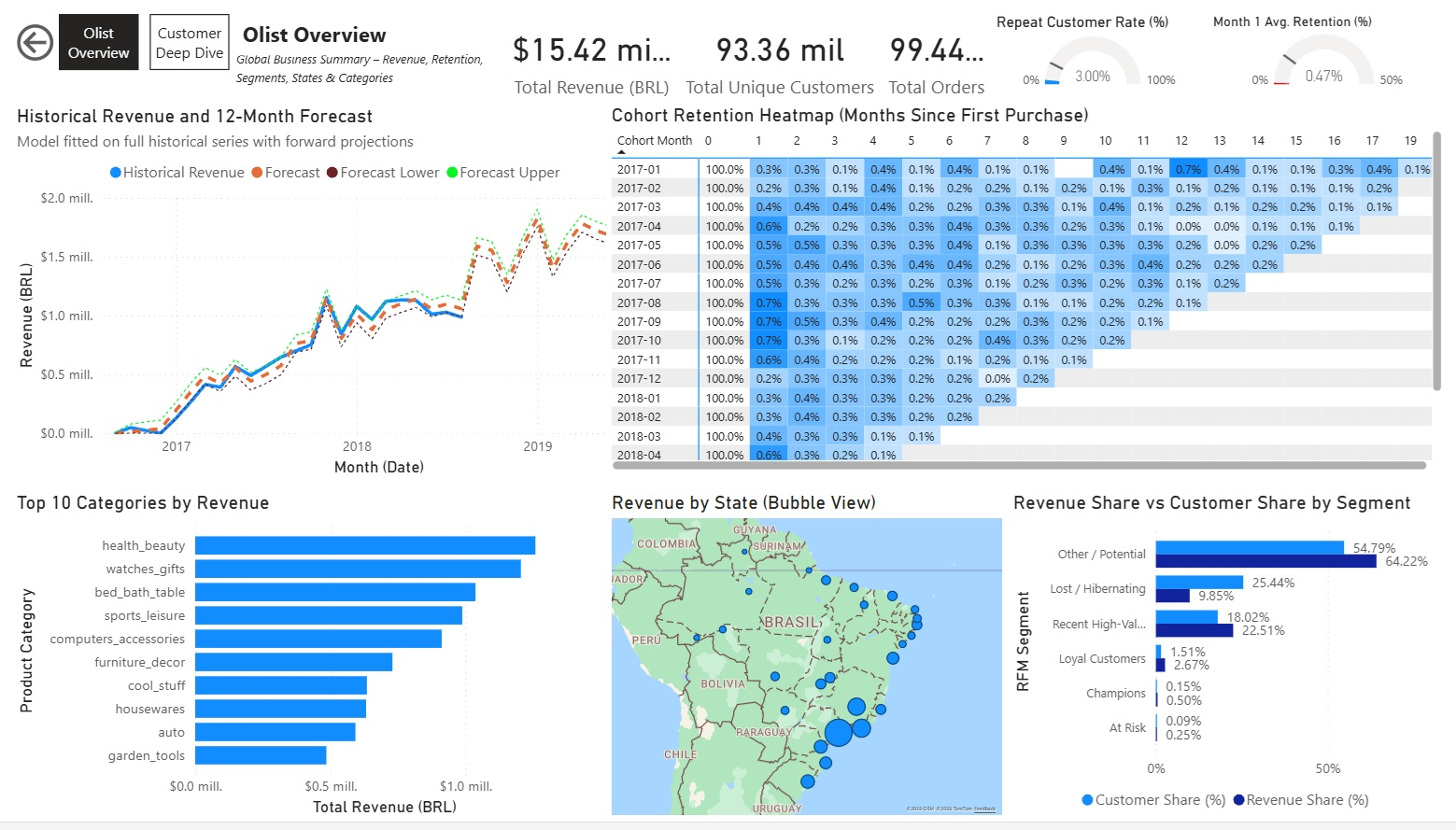
9.3. Dashboard in Power BI 
Per rendere l'analisi più interattiva e pronta per l'uso business, ho creato un dashboard in Power BI utilizzando le tabelle esportate dalla cartella processed.
Caratteristiche Principali del Dashboard:
Pagina Overview ("Olist Overview")
Riassunto di alto livello con KPI globali e visual chiave:
- Card semplici per metriche core: Ricavi Totali, Clienti Unici Totali, % Share Ricavi, % Share Clienti, Spesa Media per Cliente, Acquisti Medi per Cliente.
- Grafico a linee: Ricavi Storici + Previsione 12 Mesi
- Matrice/Heatmap: Retention dei Cohorts (Mesi dalla prima acquisto)
- Grafico a barre raggruppate: % Share Ricavi vs % Share Clienti per Segmento RFM
- Mappa Bubble: Ricavi per Stato Brasiliano
- Grafico a barre orizzontali: Top 10 Categorie per Ricavi
Nessun slicer su questa pagina per mantenerla come snapshot globale pulito.
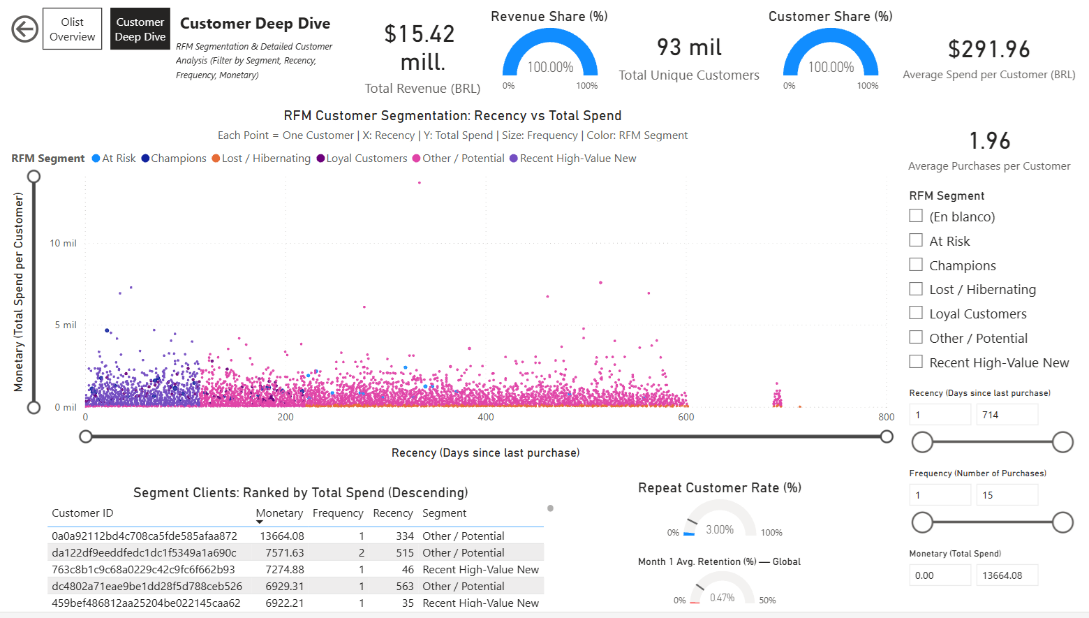
Pagina Customer Deep Dive
Focalizzata su analisi dettagliata dei clienti con interattività:
- Scatter Plot RFM: Recency vs Monetary (dimensione per Frequency, colore per Segmento)
- Tabella dinamica clienti: Filtrata e ordinata per segmento selezionato (monetary decrescente)
- Card semplici e Gauges per KPI specifici per segmento (es. % Repeat Customers, Spesa Media, ecc.)
- Multipli slicer: Segmento RFM, Range Recency, Range Frequency, Range Monetary — per filtraggio profondo e esplorazione di gruppi clienti.
Screenshots:
Pagina Olist Overview:
Pagina Customer Deep Dive:
Link al Dashboard:
Power BI Service – Olist Analytics Dashboard
Il dashboard è pubblicato su Power BI Service (account personale gratuito) e può essere condiviso via link per visualizzazione interattiva.
9.4. Conclusione del Progetto e Prossimi Passi 
Riassunto dei Risultati:
- Caricato e pulito il dataset di E-Commerce Brasiliano Olist (~100k ordini, 9 tabelle).
- Eseguito EDA profondo: vendite per stato/categoria, preferenze regionali, performance di consegna.
- Consegnata segmentazione RFM con gruppi clienti actionable e raccomandazioni.
- Analizzata retention dei cohorts → evidenziate tassi di ripetizione molto bassi e strategie di miglioramento.
- Previsione dei ricavi futuri con Prophet → identificati trend di crescita e opportunità stagionali.
- Creati visual interattivi (Plotly) e esportate tabelle per dashboarding.
Lezioni Chiave Apprese:
- Transizione riuscita da R a Python: pandas per manipolazione dati, Prophet per forecasting, Plotly per visual interattivi.
- Realtà dell'e-commerce: tasso di riacquisto molto basso (~3 %), alta dipendenza da compratori one-time.
- Importanza del contesto business: ogni analisi ha portato a raccomandazioni concrete.
- Peculiarità di Power BI: relazioni e slicer necessitano setup attento per cross-filtering.
Miglioramenti Futuri e Idee:
- Incorporare dati esterni (es. festività brasiliane, indicatori economici) per forecasting più ricco.
- Esplorare impatto dei metodi di pagamento su segmenti e retention (boleto vs carta vs rate).
- Eseguire A/B test reali su tattiche di retention (es. email win-back, sconti) se dati live disponibili.
- Scalare a modelli più avanzati (es. deep learning per serie temporali, ML per customer lifetime value).
Questo progetto dimostra competenze di analisi dati end-to-end: dai dati raw alle raccomandazioni di business, con forti capacità in Python/SQL/visualizzazione.
Grazie per avermi seguito!
9.5 Report Pubblicato e Download 
L'analisi interattiva completa è disponibile online sul mio sito web personale:
Visualizza Report Interattivo (HTML)
(Raccomandato – interattività completa, TOC cliccabile, celle codice espandibili, grafici Plotly)
Scarica Versione PDF:
Report Olist Analytics – PDF
(Export statico per lettura offline o stampa – generato dal notebook)
Entrambe le versioni si basano sullo stesso codice sorgente del Jupyter notebook disponibile nel mio repository.
Emilio Nahuel Pattini – Buenos Aires, 1 febbraio 2026