Diabetes Risk Analysis & Public Health Insights
US BRFSS 2023 • SQL • Clustering • Streamlit Dashboard • Latin America Context
Author: Emilio Nahuel Pattini
Date: April 2025
Objective: Analyze diabetes risk factors using BRFSS 2023 data (USA), build predictive models, perform clustering for population segmentation, and contextualize findings with Latin America trends and projections (PAHO & IDF data).
Project Overview
This project aims to:
- Perform exploratory data analysis (EDA) on diabetes indicators from the 2023 Behavioral Risk Factor Surveillance System (BRFSS).
- Identify key risk factors and correlations.
- Build a classification model to predict diabetes/pre-diabetes risk.
- Apply clustering to segment populations by risk profiles.
- Enrich the analysis with regional data from Latin America (prevalence trends, burden, mortality, treatment gaps).
- Provide actionable public health insights and recommendations, especially relevant for Argentina and Latin America.
Datasets
Main Dataset
- Source: CDC BRFSS 2023 (cleaned version from Kaggle)
- File:
diabetes_012_health_indicators_BRFSS2023.csv - Rows: ~261,589
- Target: Diabetes_012 (0 = no diabetes, 1 = pre-diabetes, 2 = diabetes)
- Key features: BMI, HighBP, GenHlth, PhysActivity, Age, Income, etc.
Latam Context Datasets
- IDF Diabetes Atlas – South & Central America projections (2000–2050)
File:idf_south_central_america_formatted.csv - PAHO Prevalence and Treatment Coverage (1990–2022)
File:paho_prevalence_trends.csv - PAHO Burden of Diabetes 2019 (by subregion)
File:paho_burden_2019.csv - PAHO Deaths by Country (2019)
File:paho_level_by_country.csv - PAHO Summary – Treatment Gap (1990–2022)
File:paho_diabetes_in_the_americas_summary_of_estimates.csv
- IDF Diabetes Atlas – South & Central America projections (2000–2050)
Objectives
Main Objectives
- Understand diabetes prevalence and risk factors in the US population (2023 data).
- Build and evaluate a predictive model for diabetes risk classification.
- Identify population segments with similar risk profiles using clustering.
- Compare US patterns with Latin America trends and future projections.
Technical Goals
- Demonstrate advanced SQL usage (DuckDB) for data preparation and aggregation.
- Perform complete EDA with interactive visualizations (Plotly).
- Apply supervised (classification) and unsupervised (clustering) machine learning.
- Build an interactive dashboard (Streamlit) for exploration and insights.
Table of Contents
1. Data Preparation & Cleaning
1.1. Data Preparation
import duckdb
import pandas as pd
import numpy as np
import matplotlib.pyplot as plt
import seaborn as sns
import plotly.express as px
import plotly.io as pio
pio.renderers.default = "notebook_connected"
# Configuration
pd.set_option('display.max_columns', None)
sns.set(style="whitegrid")
# Connect to DuckDB
con = duckdb.connect()
# File path
base_path = "./data/raw/"
files = {
"cdc": base_path + "diabetes_012_health_indicators_BRFSS2023.csv",
"idf": base_path + "idf_south_central_america_formatted.csv",
"paho_prevalence": base_path + "paho_prevalence_trends.csv",
"paho_burden": base_path + "paho_burden_2019.csv",
"paho_deaths_country": base_path + "paho_level_by_country.csv",
"paho_summary": base_path + "paho_diabetes_in_the_americas_summary_of_estimates.csv"
}
# Load all tables
for name, path in files.items():
con.execute(f"""
CREATE OR REPLACE TABLE {name} AS
SELECT * FROM read_csv_auto('{path}')
""")
print(f"Table '{name}' loaded.")
# Function to check basic info
def quick_check(table_name):
print(f"\n=== {table_name.upper()} ===")
count = con.execute(f"SELECT COUNT(*) AS rows FROM {table_name}").fetchone()[0]
print(f"Rows: {count:,}")
print("\nColumns:")
cols = con.execute(f"DESCRIBE {table_name}").fetchdf()
print(cols[['column_name', 'column_type']])
print("\nFirst 3 rows:")
print(con.execute(f"SELECT * FROM {table_name} LIMIT 3").fetchdf())
# Verify all tables
for name in files.keys():
quick_check(name)
# Quick view of CDC target
print("\nDiabetes_012 (CDC): Distribution")
print(con.execute("""
SELECT Diabetes_012, COUNT(*) AS count,
ROUND(COUNT(*) * 100.0 / SUM(COUNT(*)) OVER (), 2) AS percentage
FROM cdc
GROUP BY Diabetes_012
ORDER BY Diabetes_012
""").fetchdf())
Table 'cdc' loaded.
Table 'idf' loaded.
Table 'paho_prevalence' loaded.
Table 'paho_burden' loaded.
Table 'paho_deaths_country' loaded.
Table 'paho_summary' loaded.
=== CDC ===
Rows: 261,589
Columns:
column_name column_type
0 Diabetes_012 DOUBLE
1 KidneyDisease DOUBLE
2 HighBP DOUBLE
3 HighChol DOUBLE
4 CholCheck DOUBLE
5 Asthma DOUBLE
6 COPD DOUBLE
7 BMI DOUBLE
8 Smoker DOUBLE
9 Stroke DOUBLE
10 HeartDiseaseorAttack DOUBLE
11 PhysActivity DOUBLE
12 HvyAlcoholConsump DOUBLE
13 AnyHealthcare DOUBLE
14 NoDocbcCost DOUBLE
15 GenHlth DOUBLE
16 MentHlth DOUBLE
17 PhysHlth DOUBLE
18 DiffWalk DOUBLE
19 Sex DOUBLE
20 AgeGroup DOUBLE
21 Education DOUBLE
22 Income DOUBLE
First 3 rows:
Diabetes_012 KidneyDisease HighBP HighChol CholCheck Asthma COPD \
0 0.0 2.0 1.0 1.0 1.0 1.0 2.0
1 2.0 2.0 1.0 0.0 1.0 2.0 2.0
2 0.0 2.0 1.0 1.0 1.0 2.0 2.0
BMI Smoker Stroke HeartDiseaseorAttack PhysActivity \
0 22.0 1.0 0.0 0.0 1.0
1 26.0 0.0 0.0 0.0 1.0
2 30.0 0.0 0.0 0.0 1.0
HvyAlcoholConsump AnyHealthcare NoDocbcCost GenHlth MentHlth PhysHlth \
0 0.0 1.0 1.0 4.0 2.0 6.0
1 0.0 1.0 0.0 4.0 0.0 0.0
2 0.0 1.0 0.0 3.0 3.0 2.0
DiffWalk Sex AgeGroup Education Income
0 1.0 0.0 13.0 4.0 2.0
1 1.0 0.0 12.0 5.0 7.0
2 0.0 0.0 9.0 5.0 7.0
=== IDF ===
Rows: 88
Columns:
column_name column_type
0 Category VARCHAR
1 Metric VARCHAR
2 Year BIGINT
3 Value DOUBLE
First 3 rows:
Category \
0 Diabetes estimates (20-79 y)
1 Diabetes estimates (20-79 y)
2 Diabetes estimates (20-79 y)
Metric Year Value
0 People with diabetes, in 1,000s 2000 8553.3
1 Age-standardised prevalence of diabetes, % 2000 3.7
2 Proportion of people with undiagnosed diabetes, % 2000 NaN
=== PAHO_PREVALENCE ===
Rows: 180
Columns:
column_name column_type
0 Location Code VARCHAR
1 Location Name En VARCHAR
2 Indicator Name En VARCHAR
3 Age Group En VARCHAR
4 Sex En VARCHAR
5 Year BIGINT
6 Value VARCHAR
7 Value Low VARCHAR
8 Value High VARCHAR
First 3 rows:
Location Code Location Name En \
0 AMR Region of the Americas
1 AMR Region of the Americas
2 AMR Region of the Americas
Indicator Name En Age Group En Sex En \
0 Diabetes treatment coverage (current use of gl... 30+ years Both sexes
1 Diabetes treatment coverage (current use of gl... 30+ years Both sexes
2 Diabetes treatment coverage (current use of gl... 30+ years Both sexes
Year Value Value Low Value High
0 1990 42.47% 38.20% 46.90%
1 1995 44.62% 41.00% 48.20%
2 2000 46.60% 43.80% 49.50%
=== PAHO_BURDEN ===
Rows: 120
Columns:
column_name column_type
0 Iso3 VARCHAR
1 Location Name VARCHAR
2 AMRO subregions VARCHAR
3 Causename Eng VARCHAR
4 Year BIGINT
5 Sex VARCHAR
6 Age group VARCHAR
7 Measure Name En VARCHAR
8 Metric Name En VARCHAR
9 Value VARCHAR
10 Value Low VARCHAR
11 Value Up VARCHAR
First 3 rows:
Iso3 Location Name AMRO subregions \
0 AMRO Region of the Americas Region of the Americas
1 AMRO Region of the Americas Region of the Americas
2 AMRO Region of the Americas Region of the Americas
Causename Eng Year Sex \
0 Diabetes mellitus (excluding CKD due to Diabetes) 2019 Both sexes
1 Diabetes mellitus (excluding CKD due to Diabetes) 2019 Both sexes
2 Diabetes mellitus (excluding CKD due to Diabetes) 2019 Both sexes
Age group Measure Name En Metric Name En \
0 Age-standardized Deaths Rate
1 Age-standardized Disability-Adjusted Life Years (DALYs) Rate
2 Age-standardized Years Lived with Disability (YLDs) Rate
Value Value Low Value Up
0 19.64 17.26 22.02
1 1,119.49 866.64 1,423.70
2 604.86 408.1 847.76
=== PAHO_DEATHS_COUNTRY ===
Rows: 35
Columns:
column_name column_type
0 Iso3 VARCHAR
1 Quintiles classes VARCHAR
2 Causename Eng VARCHAR
3 Location Name VARCHAR
4 Measure Name En VARCHAR
5 Year BIGINT
6 Latitude (generated) DOUBLE
7 Longitude (generated) DOUBLE
8 Value Low DOUBLE
9 Value Up DOUBLE
10 Value DOUBLE
First 3 rows:
Iso3 Quintiles classes \
0 VEN Quintile 3: 40 to 60%
1 VCT Quintile 3: 40 to 60%
2 USA Quintile 1: 0 to 20%
Causename Eng \
0 Diabetes mellitus (excluding CKD due to Diabetes)
1 Diabetes mellitus (excluding CKD due to Diabetes)
2 Diabetes mellitus (excluding CKD due to Diabetes)
Location Name Measure Name En Year \
0 Venezuela, Bolivarian Republic of Deaths 2019
1 Saint Vincent and the Grenadines Deaths 2019
2 United States of America Deaths 2019
Latitude (generated) Longitude (generated) Value Low Value Up \
0 6.9830 -64.5880 30.33924 49.751212
1 13.2528 -61.1949 35.87554 50.156859
2 40.0792 -98.8164 8.34613 9.646632
Value
0 39.291483
1 42.725138
2 9.115689
=== PAHO_SUMMARY ===
Rows: 66
Columns:
column_name column_type
0 Year of Year dated BIGINT
1 Indicator Name En VARCHAR
2 % of Total Value VARCHAR
First 3 rows:
Year of Year dated Indicator Name En \
0 1990 Number of people aged 30+ years with diabetes ...
1 1991 Number of people aged 30+ years with diabetes ...
2 1992 Number of people aged 30+ years with diabetes ...
% of Total Value
0 42.36717%
1 42.77484%
2 43.18176%
Diabetes_012 (CDC): Distribution
Diabetes_012 count percentage
0 0.0 216762 82.86
1 1.0 6581 2.52
2 2.0 38246 14.62
1.2. Initial Data Cleaning
I will:
- Convert percentage strings to float
- Check for missing values
- Standardize column names (lowercase, no spaces)
- Create cleaned versions of tables if needed
# 1.2.1. PAHO Prevalence: Convert Value, Value Low, Value High a float
con.execute("""
UPDATE paho_prevalence
SET
Value = CAST(REPLACE(Value, '%', '') AS DOUBLE),
"Value Low" = CAST(REPLACE("Value Low", '%', '') AS DOUBLE),
"Value High" = CAST(REPLACE("Value High", '%', '') AS DOUBLE)
WHERE Value IS NOT NULL
""")
# Verify that they converted
print("Example after cleaning (PAHO Prevalence):")
print(con.execute("""
SELECT "Indicator Name En", Year, Value, "Value Low", "Value High"
FROM paho_prevalence
WHERE Year IN (2019, 2022)
LIMIT 10
""").fetchdf())
# 1.2.2. Rename columns for consistency
# Example for CDC: all lowercase and replace spaces/camelCase
con.execute("""
CREATE OR REPLACE TABLE cdc_clean AS
SELECT
Diabetes_012,
KidneyDisease,
HighBP,
HighChol,
CholCheck,
Asthma,
COPD,
BMI,
Smoker,
Stroke,
HeartDiseaseorAttack,
PhysActivity,
HvyAlcoholConsump,
AnyHealthcare,
NoDocbcCost,
GenHlth,
MentHlth,
PhysHlth,
DiffWalk,
Sex,
AgeGroup,
Education,
Income
FROM cdc
""")
# For IDF (previously formatted, now rename)
con.execute("""
ALTER TABLE idf RENAME COLUMN "Category" TO category;
ALTER TABLE idf RENAME COLUMN "Metric" TO metric;
ALTER TABLE idf RENAME COLUMN "Year" TO year;
ALTER TABLE idf RENAME COLUMN "Value" TO value;
""")
# General check for missing values in CDC
print("\nMissing values in CDC:")
print(con.execute("""
SELECT
column_name,
SUM(CASE WHEN column_name IS NULL THEN 1 ELSE 0 END) AS missing_count
FROM
(DESCRIBE cdc) AS cols
CROSS JOIN
(SELECT * FROM cdc LIMIT 1) AS sample
GROUP BY column_name
""").fetchdf()) # Aproximate
print("\nAll looks clean and ready for EDA.")
Example after cleaning (PAHO Prevalence):
Indicator Name En Year Value Value Low \
0 Diabetes treatment coverage (current use of gl... 2019 56.28 53.2
1 Diabetes treatment coverage (current use of gl... 2022 57.71 53.3
2 Diabetes treatment coverage (current use of gl... 2019 56.72 52.2
3 Diabetes treatment coverage (current use of gl... 2022 57.83 51.5
4 Diabetes treatment coverage (current use of gl... 2019 55.89 51.2
5 Diabetes treatment coverage (current use of gl... 2022 57.65 50.9
6 Diabetes treatment coverage (current use of gl... 2019 57.57 54.4
7 Diabetes treatment coverage (current use of gl... 2022 59.3 54.9
8 Diabetes treatment coverage (current use of gl... 2019 58.13 53.6
9 Diabetes treatment coverage (current use of gl... 2022 59.51 53.1
Value High
0 59.4
1 62.1
2 61.0
3 63.9
4 60.3
5 63.9
6 60.7
7 63.7
8 62.5
9 65.6
Missing values in CDC:
column_name missing_count
0 HighBP 0.0
1 Sex 0.0
2 Education 0.0
3 KidneyDisease 0.0
4 BMI 0.0
5 GenHlth 0.0
6 Asthma 0.0
7 Stroke 0.0
8 PhysHlth 0.0
9 PhysActivity 0.0
10 HighChol 0.0
11 CholCheck 0.0
12 COPD 0.0
13 MentHlth 0.0
14 Diabetes_012 0.0
15 Income 0.0
16 HeartDiseaseorAttack 0.0
17 HvyAlcoholConsump 0.0
18 Smoker 0.0
19 AgeGroup 0.0
20 NoDocbcCost 0.0
21 DiffWalk 0.0
22 AnyHealthcare 0.0
All looks clean and ready for EDA.
1.3. Final Data Cleaning & Standardization
Here I standardize column names (lowercase, underscores) across all tables and convert the remaining percentage column in PAHO summary.
# 1.3.1. Clean PAHO Summary: convert % of Total Value to float
con.execute("""
UPDATE paho_summary
SET "% of Total Value" = CAST(REPLACE("% of Total Value", '%', '') AS DOUBLE)
WHERE "% of Total Value" IS NOT NULL
""")
print("Example after cleaning PAHO Summary:")
print(con.execute("""
SELECT "Year of Year dated", "Indicator Name En", "% of Total Value"
FROM paho_summary
WHERE "Year of Year dated" IN (2019, 2022)
""").fetchdf())
Example after cleaning PAHO Summary: Year of Year dated Indicator Name En \ 0 2019 Number of people aged 30+ years with diabetes ... 1 2022 Number of people aged 30+ years with diabetes ... 2 2019 Number of people aged 30+ years with diabetes ... 3 2022 Number of people aged 30+ years with diabetes ... % of Total Value 0 57.56768 1 59.30143 2 42.43232 3 40.69857
# 1.3.2. Standardize column names (lowercase + underscores) for all tables
# This is to make queries easier and more consistent
# Function to rename columns in DuckDB
def standardize_columns(table_name):
cols = con.execute(f"DESCRIBE {table_name}").fetchdf()['column_name'].tolist()
for col in cols:
new_col = col.lower().replace(' ', '_').replace('(', '').replace(')', '').replace('-', '_').replace('%', 'percent')
if new_col != col:
con.execute(f"ALTER TABLE {table_name} RENAME COLUMN \"{col}\" TO {new_col}")
print(f"Standardized columns in {table_name}")
# Apply to all tables
for table in ['cdc', 'idf', 'paho_prevalence', 'paho_burden', 'paho_deaths_country', 'paho_summary']:
standardize_columns(table)
# Quick check after standardization (example for one table)
print("\nCDC columns after standardization:")
print(con.execute("DESCRIBE cdc").fetchdf()[['column_name']])
print("\nAll tables are now clean and standardized. Ready for EDA!")
Standardized columns in cdc
Standardized columns in idf
Standardized columns in paho_prevalence
Standardized columns in paho_burden
Standardized columns in paho_deaths_country
Standardized columns in paho_summary
CDC columns after standardization:
column_name
0 diabetes_012
1 kidneydisease
2 highbp
3 highchol
4 cholcheck
5 asthma
6 copd
7 bmi
8 smoker
9 stroke
10 heartdiseaseorattack
11 physactivity
12 hvyalcoholconsump
13 anyhealthcare
14 nodocbccost
15 genhlth
16 menthlth
17 physhlth
18 diffwalk
19 sex
20 agegroup
21 education
22 income
All tables are now clean and standardized. Ready for EDA!
1.4. Final Numeric Type Conversion
Here I'll convert all columns that should be numeric from VARCHAR to DOUBLE. This is to prevent repeated CASTs and ensure correct calculations.
print("Final numeric conversion check & fix...")
def safe_convert_to_double(table, column):
# Check current type
current_type = con.execute(f"""
SELECT column_type
FROM (DESCRIBE {table})
WHERE column_name = '{column}'
""").fetchone()[0]
if 'DOUBLE' in current_type.upper() or 'FLOAT' in current_type.upper():
print(f" {table}.{column} is already numeric ({current_type}) - skipping")
return
try:
# Remove commas if present (only if still string)
con.execute(f"""
UPDATE {table}
SET {column} = REPLACE({column}, ',', '')
WHERE {column} IS NOT NULL
""")
# Convert to DOUBLE
con.execute(f"""
ALTER TABLE {table}
ALTER COLUMN {column} SET DATA TYPE DOUBLE USING CAST({column} AS DOUBLE)
""")
print(f" Converted {table}.{column} → DOUBLE")
except Exception as e:
print(f" Warning on {table}.{column}: {e}")
# Apply to all relevant columns
tables_cols = [
('paho_prevalence', ['value', 'value_low', 'value_high']),
('paho_burden', ['value', 'value_low', 'value_up']),
('paho_summary', ['percent_of_total_value']),
('paho_deaths_country', ['value', 'value_low', 'value_up'])
]
for table, cols in tables_cols:
for col in cols:
safe_convert_to_double(table, col)
# Final check
print("\nFinal column types check:")
for table in ['paho_prevalence', 'paho_burden', 'paho_summary', 'paho_deaths_country']:
print(f"\n{table.upper()}:")
print(con.execute(f"DESCRIBE {table}").fetchdf()[['column_name', 'column_type']])
Final numeric conversion check & fix...
Converted paho_prevalence.value → DOUBLE
Converted paho_prevalence.value_low → DOUBLE
Converted paho_prevalence.value_high → DOUBLE
Converted paho_burden.value → DOUBLE
Converted paho_burden.value_low → DOUBLE
Converted paho_burden.value_up → DOUBLE
Converted paho_summary.percent_of_total_value → DOUBLE
paho_deaths_country.value is already numeric (DOUBLE) - skipping
paho_deaths_country.value_low is already numeric (DOUBLE) - skipping
paho_deaths_country.value_up is already numeric (DOUBLE) - skipping
Final column types check:
PAHO_PREVALENCE:
column_name column_type
0 location_code VARCHAR
1 location_name_en VARCHAR
2 indicator_name_en VARCHAR
3 age_group_en VARCHAR
4 sex_en VARCHAR
5 year BIGINT
6 value DOUBLE
7 value_low DOUBLE
8 value_high DOUBLE
PAHO_BURDEN:
column_name column_type
0 iso3 VARCHAR
1 location_name VARCHAR
2 amro_subregions VARCHAR
3 causename_eng VARCHAR
4 year BIGINT
5 sex VARCHAR
6 age_group VARCHAR
7 measure_name_en VARCHAR
8 metric_name_en VARCHAR
9 value DOUBLE
10 value_low DOUBLE
11 value_up DOUBLE
PAHO_SUMMARY:
column_name column_type
0 year_of_year_dated BIGINT
1 indicator_name_en VARCHAR
2 percent_of_total_value DOUBLE
PAHO_DEATHS_COUNTRY:
column_name column_type
0 iso3 VARCHAR
1 quintiles_classes VARCHAR
2 causename_eng VARCHAR
3 location_name VARCHAR
4 measure_name_en VARCHAR
5 year BIGINT
6 latitude_generated DOUBLE
7 longitude_generated DOUBLE
8 value_low DOUBLE
9 value_up DOUBLE
10 value DOUBLE
2. Exploratory Data Analysis (EDA)
I will explore:
- Distribution of the target variable ('Diabetes_012')
- Key demographic and health risk factors
- Relationships between features and diabetes status
- Initial context from Latin America (prevalence trends)
2.1. Visual Analysis
# 2.1 Target Distribution
target_dist = con.execute("""
SELECT
diabetes_012,
COUNT(*) AS count,
ROUND(COUNT(*) * 100.0 / SUM(COUNT(*)) OVER (), 2) AS percentage
FROM cdc
GROUP BY diabetes_012
ORDER BY diabetes_012
""").fetchdf()
# Map to readable labels
status_map = {0: 'No Diabetes', 1: 'Pre-diabetes', 2: 'Diabetes'}
target_dist['diabetes_status'] = target_dist['diabetes_012'].map(status_map)
fig_target = px.bar(
target_dist,
x='diabetes_status',
y='percentage',
color='diabetes_status',
title='Diabetes Status Distribution (BRFSS 2023)',
labels={'percentage': 'Percentage (%)'},
color_discrete_map={
'No Diabetes': '#1f77b4',
'Pre-diabetes': '#ff7f0e',
'Diabetes': '#2ca02c'
},
text='percentage'
)
fig_target.update_traces(texttemplate='%{text:.2f}%', textposition='outside')
fig_target.update_layout(
yaxis_title='Percentage of Respondents (%)',
xaxis_title='Diabetes Status',
legend_title_text='Diabetes Status',
showlegend=False # Not needed since x-axis already has labels
)
fig_target.show()
# 2.2 Age Group Distribution
age_map = {
1: '18-24', 2: '25-29', 3: '30-34', 4: '35-39',
5: '40-44', 6: '45-49', 7: '50-54', 8: '55-59',
9: '60-64', 10: '65-69', 11: '70-74', 12: '75-79', 13: '80+'
}
status_map = {0: 'No Diabetes', 1: 'Pre-diabetes', 2: 'Diabetes'}
age_diabetes = con.execute("""
SELECT agegroup, diabetes_012, COUNT(*) AS count
FROM cdc
GROUP BY agegroup, diabetes_012
""").fetchdf()
age_diabetes['age_group_label'] = age_diabetes['agegroup'].map(age_map)
age_diabetes['diabetes_status'] = age_diabetes['diabetes_012'].map(status_map)
age_diabetes['percentage'] = age_diabetes.groupby('age_group_label')['count'].transform(lambda x: x / x.sum() * 100)
fig_age = px.bar(
age_diabetes,
x='age_group_label',
y='percentage',
color='diabetes_status',
barmode='stack',
title='Diabetes Status by Age Group',
labels={'percentage': 'Percentage (%)', 'age_group_label': 'Age Group'},
color_discrete_map={
'No Diabetes': '#1f77b4', # Blue
'Pre-diabetes': '#ff7f0e', # Orange
'Diabetes': '#2ca02c' # Green
}
)
fig_age.update_layout(
legend_title_text='Diabetes Status',
yaxis_title='Percentage of People in Age Group (%)'
)
fig_age.update_xaxes(categoryorder='array', categoryarray=list(age_map.values()))
fig_age.show()
# 2.3 BMI Distribution by Diabetes Status
bmi_data = con.execute("""
SELECT diabetes_012, bmi
FROM cdc
WHERE bmi IS NOT NULL
""").fetchdf()
status_map = {0: 'No Diabetes', 1: 'Pre-diabetes', 2: 'Diabetes'}
bmi_data['diabetes_status'] = bmi_data['diabetes_012'].map(status_map)
fig_bmi = px.box(
bmi_data,
x='diabetes_status',
y='bmi',
color='diabetes_status',
title='BMI Distribution by Diabetes Status',
labels={'bmi': 'Body Mass Index (BMI)', 'diabetes_status': 'Diabetes Status'},
color_discrete_map={
'No Diabetes': '#1f77b4',
'Pre-diabetes': '#ff7f0e',
'Diabetes': '#2ca02c'
}
)
fig_bmi.update_layout(
yaxis_title='Body Mass Index (BMI)',
legend_title_text='Diabetes Status'
)
fig_bmi.show()
# 2.4 Quick look at PAHO prevalence trend (Americas)
print("\nDiabetes Prevalence Trend (Americas 18+ years, age-standardized):")
prevalence_trend = con.execute("""
SELECT
year,
AVG(value) AS avg_prevalence_percent
FROM paho_prevalence
WHERE indicator_name_en LIKE '%Prevalence of diabetes in adults aged 18+ years%'
AND "sex_en" = 'Both sexes'
AND indicator_name_en LIKE '%age-standardized%'
GROUP BY year
ORDER BY year
""").fetchdf()
print(prevalence_trend)
fig_trend = px.line(
prevalence_trend,
x='year',
y='avg_prevalence_percent',
title='Diabetes Prevalence Trend in the Americas (18+, age-standardized)',
markers=True
)
fig_trend.update_layout(yaxis_title='Prevalence (%)')
fig_trend.show()
Diabetes Prevalence Trend (Americas 18+ years, age-standardized): year avg_prevalence_percent 0 1990 7.06 1 1995 7.83 2 2000 8.51 3 2005 9.41 4 2010 10.57 5 2015 11.53 6 2019 12.32 7 2020 12.55 8 2021 12.80 9 2022 13.06
# 2.5 High Blood Pressure by Diabetes Status
status_map = {0: 'No Diabetes', 1: 'Pre-diabetes', 2: 'Diabetes'}
highbp_diabetes = con.execute("""
SELECT highbp, diabetes_012, COUNT(*) AS count
FROM cdc
GROUP BY highbp, diabetes_012
""").fetchdf()
highbp_diabetes['diabetes_status'] = highbp_diabetes['diabetes_012'].map(status_map)
highbp_diabetes['percentage'] = highbp_diabetes.groupby('highbp')['count'].transform(lambda x: x / x.sum() * 100)
fig_highbp = px.bar(
highbp_diabetes,
x='highbp',
y='percentage',
color='diabetes_status',
barmode='stack',
title='High Blood Pressure by Diabetes Status',
labels={'highbp': 'High Blood Pressure', 'percentage': 'Percentage (%)'},
color_discrete_map={
'No Diabetes': '#1f77b4',
'Pre-diabetes': '#ff7f0e',
'Diabetes': '#2ca02c'
}
)
fig_highbp.update_xaxes(tickvals=[0, 1], ticktext=['No', 'Yes'])
fig_highbp.update_layout(
legend_title_text='Diabetes Status',
yaxis_title='Percentage within each HighBP group (%)'
)
fig_highbp.show()
#2.6 General Health by Diabetes Status
status_map = {0: 'No Diabetes', 1: 'Pre-diabetes', 2: 'Diabetes'}
genhlth_diabetes = con.execute("""
SELECT genhlth, diabetes_012, COUNT(*) AS count
FROM cdc
GROUP BY genhlth, diabetes_012
""").fetchdf()
genhlth_diabetes['diabetes_status'] = genhlth_diabetes['diabetes_012'].map(status_map)
genhlth_diabetes['percentage'] = genhlth_diabetes.groupby('genhlth')['count'].transform(lambda x: x / x.sum() * 100)
fig_genhlth = px.bar(
genhlth_diabetes,
x='genhlth',
y='percentage',
color='diabetes_status',
barmode='stack',
title='Self-Reported General Health by Diabetes Status',
labels={'genhlth': 'General Health (1=Excellent → 5=Poor)', 'percentage': 'Percentage (%)'},
color_discrete_map={
'No Diabetes': '#1f77b4',
'Pre-diabetes': '#ff7f0e',
'Diabetes': '#2ca02c'
}
)
fig_genhlth.update_layout(
legend_title_text='Diabetes Status',
yaxis_title='Percentage within each Health Rating (%)'
)
fig_genhlth.show()
# 2.7 Physical Activity by Diabetes Status
physact = con.execute("""
SELECT physactivity, diabetes_012, COUNT(*) AS count
FROM cdc
GROUP BY physactivity, diabetes_012
""").fetchdf()
physact['percentage'] = physact.groupby('physactivity')['count'].transform(lambda x: x / x.sum() * 100)
physact['diabetes_status'] = physact['diabetes_012'].map(status_map)
fig_phys = px.bar(
physact,
x='physactivity',
y='percentage',
color='diabetes_status',
barmode='stack',
title='Physical Activity by Diabetes Status',
labels={'physactivity': 'Physically Active', 'percentage': 'Percentage (%)'},
color_discrete_map={'No Diabetes': '#1f77b4', 'Pre-diabetes': '#ff7f0e', 'Diabetes': '#2ca02c'}
)
fig_phys.update_xaxes(tickvals=[0, 1], ticktext=['No', 'Yes'])
fig_phys.update_layout(legend_title_text='Diabetes Status')
fig_phys.show()
# 2.8 Income Level by Diabetes Status
income_diabetes = con.execute("""
SELECT income, diabetes_012, COUNT(*) AS count
FROM cdc
GROUP BY income, diabetes_012
""").fetchdf()
income_diabetes['percentage'] = income_diabetes.groupby('income')['count'].transform(lambda x: x / x.sum() * 100)
income_diabetes['diabetes_status'] = income_diabetes['diabetes_012'].map(status_map)
fig_income = px.bar(
income_diabetes,
x='income',
y='percentage',
color='diabetes_status',
barmode='stack',
title='Income Level by Diabetes Status',
labels={'income': 'Income Level (1=Low → 8=High)', 'percentage': 'Percentage (%)'},
color_discrete_map={'No Diabetes': '#1f77b4', 'Pre-diabetes': '#ff7f0e', 'Diabetes': '#2ca02c'}
)
fig_income.update_layout(legend_title_text='Diabetes Status')
fig_income.show()
# 2.9 Correlation Heatmap
numeric_cols = ['bmi', 'highbp', 'highchol', 'physactivity', 'genhlth',
'menthlth', 'physhlth', 'diffwalk', 'agegroup', 'income']
corr_df = con.execute(f"SELECT {', '.join(numeric_cols)} FROM cdc").fetchdf().corr()
fig_corr = px.imshow(
corr_df,
text_auto='.2f',
aspect="auto",
color_continuous_scale='RdBu_r',
title='Correlation Heatmap of Key Risk Factors'
)
fig_corr.update_layout(
xaxis_title='Features',
yaxis_title='Features'
)
fig_corr.show()
2.2. Key Insights and Conclusions
1. Target Variable Distribution
- The dataset is heavily imbalanced: **82.86%** of respondents have no diabetes, **14.62%** have diabetes, and only **2.52%** are in the pre-diabetes category. - This imbalance is typical in real-world health data and will need to be handled carefully during modeling (e.g., using class weights or SMOTE).2. Strongest Risk Factors
- **BMI**: Individuals with diabetes (class 2) show a significantly higher median BMI compared to those without diabetes. Obesity appears to be one of the strongest associated factors. - **High Blood Pressure**: People with HighBP have a much higher proportion of diabetes cases. The relationship is very clear in the stacked bar chart. - **General Health**: There is a strong gradient — the worse the self-reported general health (higher GenHlth score), the higher the percentage of diabetes. - **Age**: Diabetes prevalence increases markedly with age, especially after 50–55 years old. - **Physical Activity**: Respondents who report being physically active show a lower proportion of diabetes.3. Socioeconomic Patterns
- Lower income levels are associated with higher diabetes prevalence, suggesting possible links with access to healthcare, nutrition, and prevention resources.Latin America Context
- Diabetes prevalence in the Americas (age-standardized, 18+) has been steadily increasing from ~7.1% in 1990 to ~13.1% in 2022. - IDF projections for South & Central America show a concerning rise: from 10.1% in 2024 to an estimated **11.5% in 2050**, with a large number of undiagnosed cases (~30.4% in 2024). - The burden of disease (DALYs, deaths) is particularly high in certain subregions such as Central America and the Non-Latin Caribbean.5. Main Takeaways for Public Health
- Prevention efforts should focus on **modifiable risk factors**: BMI control, blood pressure management, and promotion of physical activity. - Targeted interventions for **older adults (55+)** and **lower-income groups** could have high impact. - The growing trend in Latin America highlights the urgency of prevention policies, early screening, and improving treatment coverage (currently around 57–59% in the region).These insights will guide my next feature engineering, modeling, and clustering phases, as well as the final recommendations for public health strategies in Argentina and Latin America.
3. Feature Engineering & Advanced SQL
In this section I'll use DuckDB to create new meaningful features and perform complex transformations.
This will demonstrate efficient data preparation at scale and domain knowledge in diabetes risk factors.
Key goals:
- Create clinically meaningful variables (age groups, BMI categories, comorbidity scores, etc.)
- Engineer interaction and risk features
- Enrich the main dataset with Latam context using joins
- Prepare a clean feature set for modeling and clustering
3.1. Creating a Working Table
# 3.1 Create Clean Working Table
print("Creating clean working table 'diabetes_features' for engineering...")
con.execute("""
CREATE OR REPLACE TABLE diabetes_features AS
SELECT
diabetes_012,
bmi,
highbp,
highchol,
cholcheck,
smoker,
stroke,
heartdiseaseorattack,
physactivity,
hvyalcoholconsump,
genhlth,
menthlth,
physhlth,
diffwalk,
sex,
agegroup,
education,
income,
kidneydisease,
asthma,
copd,
anyhealthcare,
nodocbccost
FROM cdc
""")
print("Working table 'diabetes_features' created with",
con.execute("SELECT COUNT(*) FROM diabetes_features").fetchone()[0], "rows")
Creating clean working table 'diabetes_features' for engineering... Working table 'diabetes_features' created with 261589 rows
3.2. Feature Engineering
# 3.2 Feature Engineering
print("Starting feature engineering...")
con.execute("""
CREATE OR REPLACE TABLE diabetes_features AS
SELECT
*,
-- 1. Age Groups (clinically meaningful)
CASE
WHEN agegroup <= 5 THEN 'Young Adult (18-44)'
WHEN agegroup <= 8 THEN 'Middle Aged (45-59)'
WHEN agegroup <= 11 THEN 'Senior (60-74)'
ELSE 'Elderly (75+)'
END AS age_group_cat,
-- 2. BMI Categories (WHO standard)
CASE
WHEN bmi < 18.5 THEN 'Underweight'
WHEN bmi < 25.0 THEN 'Normal'
WHEN bmi < 30.0 THEN 'Overweight'
WHEN bmi < 35.0 THEN 'Obese Class I'
WHEN bmi < 40.0 THEN 'Obese Class II'
ELSE 'Obese Class III'
END AS bmi_category,
-- 3. Comorbidity Count
(highbp + highchol + kidneydisease + stroke + heartdiseaseorattack + asthma + copd)::INTEGER AS comorbidity_count,
-- 4. Risk Score (simple additive)
(highbp + highchol + (bmi >= 30)::INTEGER + (physactivity = 0)::INTEGER +
(genhlth >= 4)::INTEGER + (diffwalk = 1)::INTEGER)::INTEGER AS diabetes_risk_score,
-- 5. Age + BMI Interaction (high risk combination)
CASE
WHEN agegroup >= 9 AND bmi >= 30 THEN 'High Risk: Senior + Obese'
WHEN agegroup >= 7 AND bmi >= 30 THEN 'Moderate Risk: Middle-age + Obese'
ELSE 'Standard Risk'
END AS age_bmi_risk_group,
-- 6. Lifestyle Score (higher = better)
(physactivity + (hvyalcoholconsump = 0)::INTEGER + (smoker = 0)::INTEGER)::INTEGER AS lifestyle_score
FROM diabetes_features
""")
print("Feature engineering completed. New features added.")
print("\nSample of engineered features:")
print(con.execute("""
SELECT diabetes_012, age_group_cat, bmi_category, comorbidity_count,
diabetes_risk_score, age_bmi_risk_group, lifestyle_score
FROM diabetes_features
LIMIT 8
""").fetchdf())
Starting feature engineering... Feature engineering completed. New features added. Sample of engineered features: diabetes_012 age_group_cat bmi_category comorbidity_count \ 0 0.0 Elderly (75+) Normal 7 1 2.0 Elderly (75+) Overweight 7 2 0.0 Senior (60-74) Obese Class I 8 3 0.0 Elderly (75+) Obese Class I 7 4 2.0 Elderly (75+) Normal 9 5 0.0 Middle Aged (45-59) Obese Class III 8 6 0.0 Senior (60-74) Obese Class I 6 7 0.0 Elderly (75+) Normal 6 diabetes_risk_score age_bmi_risk_group lifestyle_score 0 4 Standard Risk 2 1 3 Standard Risk 3 2 3 High Risk: Senior + Obese 3 3 5 High Risk: Senior + Obese 2 4 2 Standard Risk 2 5 3 Moderate Risk: Middle-age + Obese 3 6 2 High Risk: Senior + Obese 2 7 1 Standard Risk 1
3.3. Feature Exploration
Here I'll analyze how the newly engineered features relate to diabetes status.
# 3.3 Feature Exploration
print("=== Feature Exploration: New Variables vs Diabetes Status ===\n")
# 1. Age Group Category vs Diabetes Prevalence
print("1. Age Group Category vs Diabetes Prevalence:")
print(con.execute("""
SELECT
age_group_cat,
COUNT(*) AS total_count,
SUM(CASE WHEN diabetes_012 = 2 THEN 1 ELSE 0 END) AS diabetes_cases,
ROUND(100.0 * SUM(CASE WHEN diabetes_012 = 2 THEN 1 ELSE 0 END) / COUNT(*), 2) AS diabetes_pct
FROM diabetes_features
GROUP BY age_group_cat
ORDER BY diabetes_pct DESC
""").fetchdf())
# 2. BMI Category vs Diabetes Prevalence
print("\n2. BMI Category vs Diabetes Prevalence:")
print(con.execute("""
SELECT
bmi_category,
COUNT(*) AS total_count,
SUM(CASE WHEN diabetes_012 = 2 THEN 1 ELSE 0 END) AS diabetes_cases,
ROUND(100.0 * SUM(CASE WHEN diabetes_012 = 2 THEN 1 ELSE 0 END) / COUNT(*), 2) AS diabetes_pct
FROM diabetes_features
GROUP BY bmi_category
ORDER BY
CASE bmi_category
WHEN 'Underweight' THEN 1
WHEN 'Normal' THEN 2
WHEN 'Overweight' THEN 3
WHEN 'Obese Class I' THEN 4
WHEN 'Obese Class II' THEN 5
WHEN 'Obese Class III' THEN 6
END
""").fetchdf())
# 3. Comorbidity Count and Risk Score by Diabetes Status
print("\n3. Average Comorbidities and Risk Score by Diabetes Status:")
print(con.execute("""
SELECT
diabetes_012,
ROUND(AVG(comorbidity_count), 2) AS avg_comorbidities,
ROUND(AVG(diabetes_risk_score), 2) AS avg_risk_score,
ROUND(AVG(lifestyle_score), 2) AS avg_lifestyle_score
FROM diabetes_features
GROUP BY diabetes_012
ORDER BY diabetes_012
""").fetchdf())
# 4. High-Risk Age + BMI Groups
print("\n4. Age + BMI Risk Groups vs Diabetes Prevalence:")
print(con.execute("""
SELECT
age_bmi_risk_group,
COUNT(*) AS total_count,
ROUND(100.0 * SUM(CASE WHEN diabetes_012 = 2 THEN 1 ELSE 0 END) / COUNT(*), 2) AS diabetes_pct
FROM diabetes_features
GROUP BY age_bmi_risk_group
ORDER BY diabetes_pct DESC
""").fetchdf())
=== Feature Exploration: New Variables vs Diabetes Status ===
1. Age Group Category vs Diabetes Prevalence:
age_group_cat total_count diabetes_cases diabetes_pct
0 Elderly (75+) 42191 8990.0 21.31
1 Senior (60-74) 88039 17700.0 20.10
2 Middle Aged (45-59) 64257 8824.0 13.73
3 Young Adult (18-44) 67102 2732.0 4.07
2. BMI Category vs Diabetes Prevalence:
bmi_category total_count diabetes_cases diabetes_pct
0 Underweight 3495 208.0 5.95
1 Normal 64682 4464.0 6.90
2 Overweight 93432 11392.0 12.19
3 Obese Class I 58433 11045.0 18.90
4 Obese Class II 24696 6079.0 24.62
5 Obese Class III 16851 5058.0 30.02
3. Average Comorbidities and Risk Score by Diabetes Status:
diabetes_012 avg_comorbidities avg_risk_score avg_lifestyle_score
0 0.0 6.64 1.54 2.35
1 1.0 7.08 2.53 2.22
2 2.0 7.28 3.06 2.13
4. Age + BMI Risk Groups vs Diabetes Prevalence:
age_bmi_risk_group total_count diabetes_pct
0 High Risk: Senior + Obese 46214 30.81
1 Moderate Risk: Middle-age + Obese 20456 23.27
2 Standard Risk 194919 9.88
3.4. Feature Engineering Summary
Key engineered features and their relationship with diabetes:
- Age Group: Strong positive correlation with age. Elderly (75+) show 21.31% diabetes prevalence.
- BMI Category: Very strong predictor. Obesity Class III has 30.02% diabetes rate vs 6.90% in Normal weight.
- Age + BMI Risk Group: Highest risk group ("High Risk: Senior + Obese") has 30.81% diabetes prevalence.
- Comorbidity Count and Diabetes Risk Score: Both increase with diabetes status.
- Lifestyle Score: Slightly lower in people with diabetes.
These features capture important clinical and behavioral dimensions and will be used for modeling and clustering.
3.5. Final Modeling Table Creation
Here I create a final clean table diabetes_model_ready containing both original and engineered features, ready for modeling and clustering.
# 3.5 Create Final Modeling Table
print("Creating final modeling table...")
con.execute("""
CREATE OR REPLACE TABLE diabetes_model_ready AS
SELECT
diabetes_012 AS target,
-- Original features
bmi,
highbp,
highchol,
physactivity,
genhlth,
diffwalk,
agegroup,
income,
sex,
-- Engineered features
age_group_cat,
bmi_category,
comorbidity_count,
diabetes_risk_score,
age_bmi_risk_group,
lifestyle_score,
-- One-hot / dummy ready (we'll use these in modeling)
CASE WHEN bmi_category = 'Obese Class III' THEN 1 ELSE 0 END AS obese_class_iii,
CASE WHEN age_group_cat IN ('Senior (60-74)', 'Elderly (75+)') THEN 1 ELSE 0 END AS senior_or_elderly,
CASE WHEN highbp = 1 AND highchol = 1 THEN 1 ELSE 0 END AS has_metabolic_risk
FROM diabetes_features
""")
print("Final modeling table 'diabetes_model_ready' created with",
con.execute("SELECT COUNT(*) FROM diabetes_model_ready").fetchone()[0], "rows")
print("\nColumns ready for modeling:")
print(con.execute("DESCRIBE diabetes_model_ready").fetchdf()['column_name'].tolist())
Creating final modeling table... Final modeling table 'diabetes_model_ready' created with 261589 rows Columns ready for modeling: ['target', 'bmi', 'highbp', 'highchol', 'physactivity', 'genhlth', 'diffwalk', 'agegroup', 'income', 'sex', 'age_group_cat', 'bmi_category', 'comorbidity_count', 'diabetes_risk_score', 'age_bmi_risk_group', 'lifestyle_score', 'obese_class_iii', 'senior_or_elderly', 'has_metabolic_risk']
4. Predictive Modeling
I will build classification models to predict diabetes risk using the features engineered in the previous section.
Goals
- Establish a strong baseline model - Evaluate performance using appropriate metrics for imbalanced health data - Identify the most important features - Compare different algorithms (Logistic Regression vs Random Forest)I will use the diabetes_model_ready table created in the previous section.
4.1. Multi-class Approach (Initial Attempt)
I first tried to predict three separate classes:
- 0 = No Diabetes
- 1 = Pre-diabetes
- 2 = Diabetes
The models performed poorly, especially on the minority class (pre-diabetes), mainly due to severe class imbalance (82.86% No Diabetes, 2.52% Pre-diabetes, 14.62% Diabetes).
After reviewing the results, I decided to simplify the problem.
# 4.1.1 Data Preparation for Multi-class modeling
from sklearn.model_selection import train_test_split
print("=== Preparing Data for Modeling ===\n")
# 1. Load the table
df = con.execute("SELECT * FROM diabetes_model_ready").fetchdf()
# 2. One-Hot Encode all categorical columns
categorical_cols = ['age_group_cat', 'bmi_category', 'age_bmi_risk_group']
df_encoded = pd.get_dummies(df, columns=categorical_cols, drop_first=True)
print(f"Shape after One-Hot Encoding: {df_encoded.shape}")
print(f"Categorical columns encoded: {categorical_cols}")
# 3. Prepare X and y
X = df_encoded.drop(columns=['target'])
y = df_encoded['target']
# 4. Train-Test Split
X_train, X_test, y_train, y_test = train_test_split(
X, y, test_size=0.20, random_state=42, stratify=y
)
print(f"Training samples: {X_train.shape[0]:,}")
print(f"Test samples: {X_test.shape[0]:,}")
print(f"Class distribution in training set:\n{y_train.value_counts(normalize=True).round(4)*100}")
=== Preparing Data for Modeling === Shape after One-Hot Encoding: (261589, 26) Categorical columns encoded: ['age_group_cat', 'bmi_category', 'age_bmi_risk_group'] Training samples: 209,271 Test samples: 52,318 Class distribution in training set: target 0.0 82.86 2.0 14.62 1.0 2.52 Name: proportion, dtype: float64
# 4.1.2 Multi-class Modeling (Logistic Regression + Random Forest + XGBoost)
from sklearn.linear_model import LogisticRegression
from sklearn.ensemble import RandomForestClassifier
from xgboost import XGBClassifier
from sklearn.metrics import classification_report, confusion_matrix, f1_score
print("=== Training Multiple Models ===\n")
models = {
"Logistic Regression": LogisticRegression(max_iter=1000, class_weight='balanced', random_state=42, n_jobs=-1),
"Random Forest": RandomForestClassifier(n_estimators=300, class_weight='balanced', random_state=42, n_jobs=-1),
"XGBoost": XGBClassifier(n_estimators=300, learning_rate=0.1, max_depth=6,
subsample=0.8, colsample_bytree=0.8, random_state=42,
eval_metric='mlogloss', n_jobs=-1)
}
for name, model in models.items():
print(f"Training {name}...")
model.fit(X_train, y_train)
y_pred = model.predict(X_test)
print(f"\n{name} Classification Report:")
print(classification_report(y_test, y_pred, digits=4))
# F1-score for diabetes class (class 2) - most important metric
f1_diabetes = f1_score(y_test, y_pred, labels=[2], average='macro')
print(f"F1-score for Diabetes class (2): {f1_diabetes:.4f}")
print("-" * 60)
=== Training Multiple Models ===
Training Logistic Regression...
Logistic Regression Classification Report:
precision recall f1-score support
0.0 0.9421 0.6324 0.7568 43353
1.0 0.0386 0.2682 0.0674 1316
2.0 0.3354 0.6168 0.4345 7649
accuracy 0.6210 52318
macro avg 0.4387 0.5058 0.4196 52318
weighted avg 0.8307 0.6210 0.6923 52318
F1-score for Diabetes class (2): 0.4345
------------------------------------------------------------
Training Random Forest...
Random Forest Classification Report:
precision recall f1-score support
0.0 0.8552 0.8912 0.8728 43353
1.0 0.0255 0.0236 0.0245 1316
2.0 0.3361 0.2603 0.2934 7649
accuracy 0.7771 52318
macro avg 0.4056 0.3917 0.3969 52318
weighted avg 0.7584 0.7771 0.7668 52318
F1-score for Diabetes class (2): 0.2934
------------------------------------------------------------
Training XGBoost...
XGBoost Classification Report:
precision recall f1-score support
0.0 0.8488 0.9783 0.9090 43353
1.0 0.0000 0.0000 0.0000 1316
2.0 0.5544 0.1700 0.2602 7649
accuracy 0.8355 52318
macro avg 0.4677 0.3828 0.3897 52318
weighted avg 0.7844 0.8355 0.7912 52318
F1-score for Diabetes class (2): 0.2602
------------------------------------------------------------
4.2. Binary Classification (Final Approach)
Given the strong imbalance and limited predictive power on pre-diabetes, I simplified the problem to binary classification:
- Class 0: No Diabetes
- Class 1: Pre-diabetes or Diabetes (any diabetes risk)
This approach is more practical for real-world screening and produced significantly better results.
4.2.1. Data Preparation for Binary Classification
I created the binary target and applied One-Hot Encoding to the categorical variables (age_group_cat, bmi_category, age_bmi_risk_group).
# 4.2.1 Binary Classification: No Diabetes vs Any Diabetes Risk
print("=== Binary Classification: No Diabetes vs Any Diabetes Risk ===\n")
# Load fresh data
df = con.execute("SELECT * FROM diabetes_model_ready").fetchdf()
# Create binary target
df['target_binary'] = df['target'].apply(lambda x: 0 if x == 0 else 1)
# One-Hot Encoding for categorical columns
categorical_cols = ['age_group_cat', 'bmi_category', 'age_bmi_risk_group']
df_encoded = pd.get_dummies(df, columns=categorical_cols, drop_first=True)
X = df_encoded.drop(columns=['target', 'target_binary'])
y = df_encoded['target_binary']
# Train-test split
X_train, X_test, y_train, y_test = train_test_split(
X, y, test_size=0.20, random_state=42, stratify=y
)
print(f"Training samples: {X_train.shape[0]:,}")
print(f"Test samples: {X_test.shape[0]:,}")
print(f"Positive class (Any diabetes risk) percentage: {y.mean():.2%}\n")
=== Binary Classification: No Diabetes vs Any Diabetes Risk === Training samples: 209,271 Test samples: 52,318 Positive class (Any diabetes risk) percentage: 17.14%
4.2.2. Modeling Results
Logistic Regression
# 4.2.2.1 Logistic Regression
print("Training Logistic Regression (Binary)...")
model_lr = LogisticRegression(max_iter=1000, class_weight='balanced', random_state=42, n_jobs=-1)
model_lr.fit(X_train, y_train)
y_pred_lr = model_lr.predict(X_test)
print("Logistic Regression Results:")
print(classification_report(y_test, y_pred_lr, digits=4))
Training Logistic Regression (Binary)...
Logistic Regression Results:
precision recall f1-score support
0 0.9329 0.7014 0.8007 43353
1 0.3436 0.7561 0.4725 8965
accuracy 0.7107 52318
macro avg 0.6383 0.7287 0.6366 52318
weighted avg 0.8319 0.7107 0.7445 52318
Random Forest
# 4.2.2.2 Random Forest
print("\nTraining Random Forest (Binary)...")
model_rf = RandomForestClassifier(n_estimators=300, class_weight='balanced', random_state=42, n_jobs=-1)
model_rf.fit(X_train, y_train)
y_pred_rf = model_rf.predict(X_test)
print("Random Forest Results:")
print(classification_report(y_test, y_pred_rf, digits=4))
Training Random Forest (Binary)...
Random Forest Results:
precision recall f1-score support
0 0.8591 0.8956 0.8770 43353
1 0.3646 0.2898 0.3229 8965
accuracy 0.7918 52318
macro avg 0.6119 0.5927 0.6000 52318
weighted avg 0.7744 0.7918 0.7820 52318
XGBoost
# 4.2.2.3 XGBoost
print("\nTraining XGBoost (Binary)...")
model_xgb = XGBClassifier(
n_estimators=300,
learning_rate=0.1,
max_depth=6,
subsample=0.8,
colsample_bytree=0.8,
random_state=42,
eval_metric='logloss',
n_jobs=-1
)
model_xgb.fit(X_train, y_train)
y_pred_xgb = model_xgb.predict(X_test)
print("XGBoost Results:")
print(classification_report(y_test, y_pred_xgb, digits=4))
Training XGBoost (Binary)...
XGBoost Results:
precision recall f1-score support
0 0.8517 0.9716 0.9077 43353
1 0.5694 0.1816 0.2754 8965
accuracy 0.8362 52318
macro avg 0.7105 0.5766 0.5915 52318
weighted avg 0.8033 0.8362 0.7993 52318
4.2.3. Model Comparison
Model Comparison and Insights
- Logistic Regression achieved the best recall (75.61%) for the positive class (any diabetes risk). This means it is good at identifying people who are at risk, even if it sometimes gives false alarms.
- XGBoost had the highest overall accuracy (83.62%) and best precision, but missed many true cases (low recall).
- Random Forest performed in between but was not the strongest in any key metric.
Chosen Model: Logistic Regression — because in public health screening, it is more important to catch as many people at risk as possible (high recall) than to be very precise.
These results show that my engineered features (especially BMI, age, income, and comorbidity count) contain useful predictive signal for diabetes risk.
4.2.4. Feature Importance Analysis
Understanding which features contribute most to the prediction is crucial for interpretability and public health recommendations.
# 4.2.4 Feature Importance (XGBoost)
# Get feature importance from XGBoost
importances = model_xgb.feature_importances_
feature_names = X_train.columns
feat_imp = pd.DataFrame({
'feature': feature_names,
'importance': importances
}).sort_values('importance', ascending=False).head(15)
print("Top 15 Most Important Features (XGBoost):")
print(feat_imp)
# Plot
plt.figure(figsize=(10, 8))
plt.barh(feat_imp['feature'], feat_imp['importance'])
plt.xlabel('Importance Score')
plt.title('Top 15 Feature Importance - XGBoost Model')
plt.gca().invert_yaxis()
plt.tight_layout()
plt.show()
Top 15 Most Important Features (XGBoost):
feature importance
10 diabetes_risk_score 0.368261
17 age_group_cat_Young Adult (18-44) 0.081003
13 senior_or_elderly 0.068727
4 genhlth 0.053791
24 age_bmi_risk_group_Standard Risk 0.049790
6 agegroup 0.037466
14 has_metabolic_risk 0.036997
20 bmi_category_Obese Class III 0.032434
1 highbp 0.030059
3 physactivity 0.022631
8 sex 0.021122
12 obese_class_iii 0.021052
18 bmi_category_Obese Class I 0.018625
11 lifestyle_score 0.016660
0 bmi 0.016236

Top 5 Most Important Features:
- diabetes_risk_score (0.368) — My engineered composite score is the strongest predictor
- Being a Young Adult (protective factor)
- senior_or_elderly (age 60+)
- genhlth (self-reported general health)
- age_bmi_risk_group_Standard Risk
This confirms that the feature engineering added significant value to the model.
Practical Application
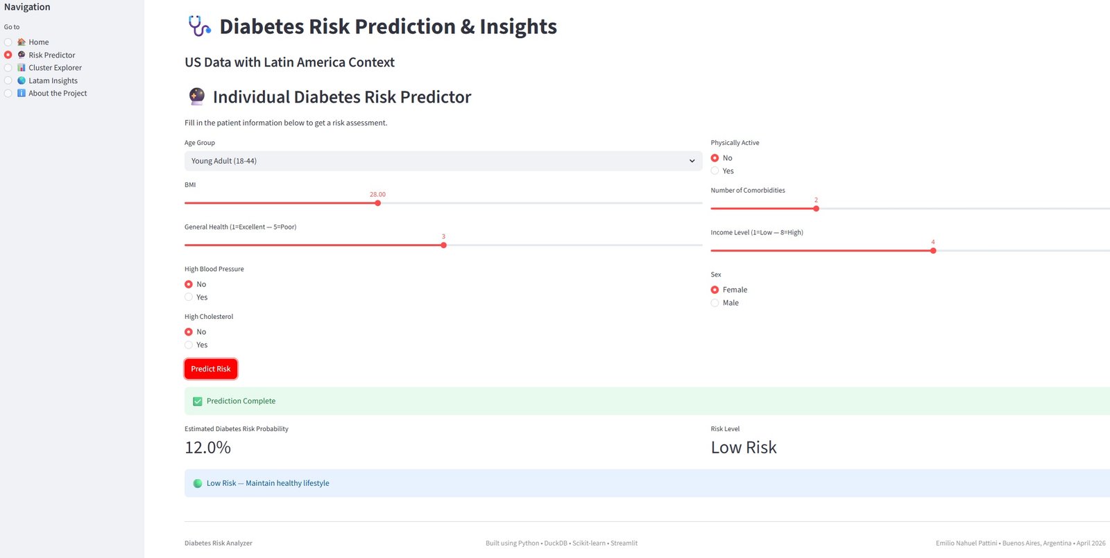
This model can be used as a Diabetes Risk Screening Tool:
- Healthcare providers can input patient data to estimate risk level.
- Public health organizations could use it to prioritize screening campaigns in high-risk groups (older adults, obese individuals, lower-income populations).
- A simplified web/app version could allow individuals to do a quick self-assessment.
Example Use Case:
A 62-year-old patient with BMI 32, high blood pressure, and poor self-reported health would be flagged as high risk, prompting earlier glucose testing and lifestyle intervention.
4.2.5. Model Demonstration with Example Patients
To illustrate how the model could be used in practice, I tested it on five realistic patient profiles.
# 4.2.5 Model Demonstration with Example Patients
print("=== Model Demonstration with Example Patients ===\n")
print("Using Logistic Regression (best recall model)\n")
# Create realistic patient profiles
examples = pd.DataFrame({
'bmi': [22.5, 27.8, 28.0, 34.5, 31.2],
'highbp': [0, 0, 1, 1, 1],
'highchol': [0, 0, 0, 1, 1],
'physactivity': [1, 0, 1, 0, 0],
'genhlth': [2, 3, 3, 4, 4],
'diffwalk': [0, 0, 0, 1, 0],
'agegroup': [4, 5, 8, 11, 10],
'income': [6, 7, 4, 3, 5],
'sex': [0, 1, 1, 0, 1],
'age_group_cat': ['Young Adult (18-44)', 'Young Adult (18-44)',
'Middle Aged (45-59)', 'Senior (60-74)', 'Senior (60-74)'],
'bmi_category': ['Normal', 'Overweight', 'Overweight',
'Obese Class I', 'Obese Class I'],
'comorbidity_count': [1, 2, 2, 5, 4],
'diabetes_risk_score': [2, 5, 4, 7, 6],
'age_bmi_risk_group': ['Standard Risk', 'Standard Risk',
'Standard Risk', 'High Risk: Senior + Obese',
'Moderate Risk: Middle-age + Obese'],
'lifestyle_score': [3, 1, 2, 1, 2],
'obese_class_iii': [0, 0, 0, 0, 0],
'senior_or_elderly': [0, 0, 0, 1, 1],
'has_metabolic_risk': [0, 0, 0, 1, 1]
})
# One-hot encode
examples_encoded = pd.get_dummies(examples,
columns=['age_group_cat', 'bmi_category', 'age_bmi_risk_group'],
drop_first=True)
for col in X_train.columns:
if col not in examples_encoded.columns:
examples_encoded[col] = 0
examples_encoded = examples_encoded[X_train.columns]
# Predictions
probabilities = model_lr.predict_proba(examples_encoded)[:, 1]
predictions = model_lr.predict(examples_encoded)
# Display
demo_results = examples.copy()
demo_results['Predicted Risk'] = ['Low Risk' if p == 0 else 'High Risk' for p in predictions]
demo_results['Risk Probability (%)'] = (probabilities * 100).round(1)
print(demo_results[[
'age_group_cat',
'bmi_category',
'genhlth',
'highbp',
'physactivity',
'Predicted Risk',
'Risk Probability (%)'
]].to_string(index=False))
=== Model Demonstration with Example Patients ===
Using Logistic Regression (best recall model)
age_group_cat bmi_category genhlth highbp physactivity Predicted Risk Risk Probability (%)
Young Adult (18-44) Normal 2 0 1 Low Risk 4.9
Young Adult (18-44) Overweight 3 0 0 Low Risk 12.6
Middle Aged (45-59) Overweight 3 1 1 High Risk 63.6
Senior (60-74) Obese Class I 4 1 0 High Risk 87.1
Senior (60-74) Obese Class I 4 1 0 High Risk 86.7
Interpretation:
The model behaves logically in most cases. Seniors with obesity and poor general health are correctly classified as high risk (86–87% probability). A middle-aged person with overweight and high blood pressure is also flagged as high risk.
However, the model remains relatively conservative with younger adults — even an overweight young adult with low physical activity is assigned only 12.6% risk. This suggests age is a very strong factor in the current model. In a real deployment, this could be adjusted depending on whether higher sensitivity (catching more cases) or higher specificity is preferred.
5. Clustering & Population Segmentation
I'll apply unsupervised learning (K-Means) to segment individuals into distinct risk groups based on their characteristics.
This allows to identify homogeneous subgroups and provide more targeted public health recommendations.
5.1. Choosing the Number of Clusters
Below, I use the Elbow Method to determine the optimal number of clusters. The inertia plot showed a reasonable bend around 4 clusters, which I adopted for interpretability.
# 5.1 Choosing the Number of Clusters - Clustering & Population Segmentation
from sklearn.cluster import KMeans
from sklearn.preprocessing import StandardScaler
import plotly.express as px
print("=== Clustering Analysis ===\n")
# Select features for clustering (numeric + encoded)
cluster_features = ['bmi', 'agegroup', 'genhlth', 'highbp', 'highchol',
'physactivity', 'comorbidity_count', 'diabetes_risk_score',
'lifestyle_score', 'senior_or_elderly', 'has_metabolic_risk']
X_cluster = X[cluster_features].copy() # Using the encoded X from previous section
# Standardize the data (this is important for K-Means)
scaler = StandardScaler()
X_scaled = scaler.fit_transform(X_cluster)
# Determine optimal number of clusters using Elbow method
inertia = []
for k in range(1, 10):
kmeans = KMeans(n_clusters=k, random_state=42, n_init=10)
kmeans.fit(X_scaled)
inertia.append(kmeans.inertia_)
fig_elbow = px.line(x=range(1,10), y=inertia, markers=True,
title='Elbow Method for Optimal Number of Clusters',
labels={'x': 'Number of Clusters (k)', 'y': 'Inertia'})
fig_elbow.show()
# Choose k=4 based on elbow + interpretability
kmeans = KMeans(n_clusters=4, random_state=42, n_init=10)
clusters = kmeans.fit_predict(X_scaled)
# Add cluster labels to the original dataframe
df_clustered = df_encoded.copy()
df_clustered['cluster'] = clusters
print("Cluster distribution:")
print(df_clustered['cluster'].value_counts().sort_index())
# Analyze clusters: Mean values per cluster
cluster_profile = df_clustered.groupby('cluster').mean().round(2)
print("\nCluster Profiles (mean values):")
print(cluster_profile[['bmi', 'agegroup', 'genhlth', 'highbp', 'comorbidity_count',
'diabetes_risk_score', 'lifestyle_score', 'target']])
=== Clustering Analysis ===
Cluster distribution:
cluster
0 95187
1 66017
2 37846
3 62539
Name: count, dtype: int64
Cluster Profiles (mean values):
bmi agegroup genhlth highbp comorbidity_count \
cluster
0 28.19 4.89 2.26 0.15 6.18
1 30.33 9.72 2.97 1.00 7.97
2 30.88 8.37 3.10 0.35 6.39
3 26.96 10.67 2.33 0.31 6.51
diabetes_risk_score lifestyle_score target
cluster
0 0.81 2.61 0.10
1 3.33 2.16 0.64
2 2.73 1.46 0.39
3 1.08 2.55 0.26
5.2. Cluster Analysis
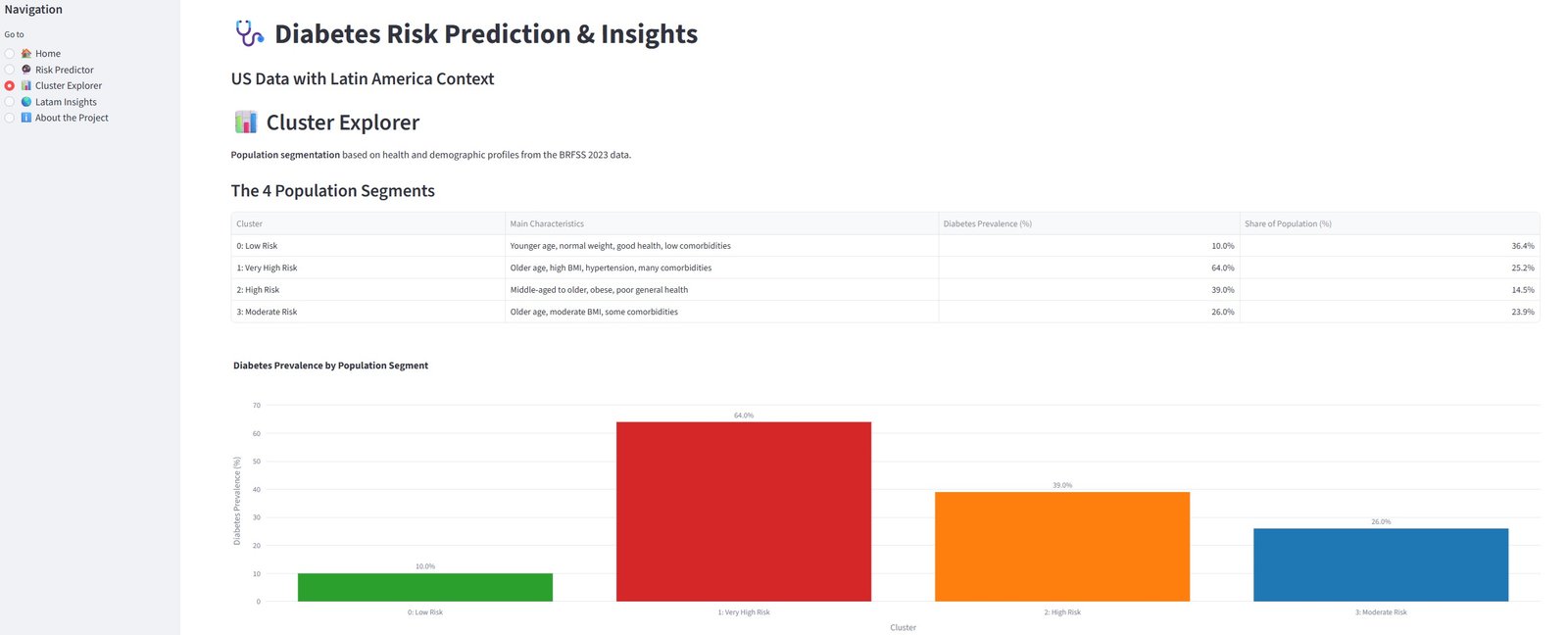
As we can see above, I obtained the following four clusters:
Cluster Distribution:
- Cluster 0: 95,187 people (36.4%)
- Cluster 1: 66,017 people (25.2%)
- Cluster 2: 37,846 people (14.5%)
- Cluster 3: 62,539 people (23.9%)
5.3. Cluster Profiles and Interpretation
I identified 4 distinct population segments based on their health characteristics.
| Cluster | Number of People | Main Characteristics | Diabetes Prevalence (%) | Risk Level | Recommendation |
|---|---|---|---|---|---|
| 0 | 95,187 | Young adults, normal weight, good general health, low comorbidities | 10.0% | Low Risk | General prevention |
| 1 | 66,017 | Older adults, high BMI, hypertension, multiple comorbidities | 64.0% | Very High Risk | Priority screening & intensive intervention |
| 2 | 37,846 | Middle-aged to older, obese, poor self-reported health | 39.0% | High Risk | Targeted lifestyle programs |
| 3 | 62,539 | Older adults, moderate BMI, some comorbidities | 26.0% | Moderate Risk | Preventive education & regular monitoring |
# 5.3 Cluster Profiles and Interpretation - Visualization
# Create a clean summary for plotting
viz_data = pd.DataFrame({
'Cluster Profile': [
'0: Low Risk (Young, healthy)',
'1: Very High Risk (Older, obese, comorbidities)',
'2: High Risk (Obese, poor health)',
'3: Moderate Risk (Older, moderate BMI)'
],
'Diabetes Prevalence (%)': [10.0, 64.0, 39.0, 26.0],
'Size (n)': [95187, 66017, 37846, 62539]
})
fig = px.bar(
viz_data,
x='Cluster Profile',
y='Diabetes Prevalence (%)',
text='Diabetes Prevalence (%)',
title='Diabetes Prevalence by Population Segment',
color='Cluster Profile',
color_discrete_sequence=['#2ca02c', '#d62728', '#ff7f0e', '#1f77b4']
)
fig.update_traces(texttemplate='%{text:.1f}%', textposition='outside')
fig.update_layout(
yaxis_title='Diabetes Prevalence (%)',
xaxis_title='Cluster Profile',
showlegend=False,
height=550
)
fig.show()
Key Insights:
- Cluster 1 is the highest-risk group (64% diabetes prevalence). It consists mainly of older individuals with obesity, hypertension, and multiple comorbidities. This group should be prioritized for aggressive screening and intervention.
- Cluster 0 represents the healthiest segment — mostly younger people with good lifestyle habits and low risk.
- Cluster 2 shows that obesity combined with poor self-reported health significantly increases risk, even in middle age.
- Age and BMI continue to be dominant drivers of risk segmentation, reinforcing findings from the EDA and modeling phases.
These clusters provide actionable insights for public health policy in Argentina and Latin America. For example, resources could be focused on Cluster 1 ("High-Risk Obese Seniors") through community screening programs and lifestyle interventions.
6. Latam Context & Comparisons
To make the analysis more relevant to Argentina and Latin America, I enriched the US-based BRFSS findings with regional data from PAHO and the IDF Diabetes Atlas.
6.1. Key Latam Indicators (South & Central America)
| Indicator | 2024 Value | 2050 Projection | Observation |
|---|---|---|---|
| Age-standardised prevalence | 10.1% | 11.5% | Steady increase expected |
| People with diabetes | 35.4 million | 51.5 million | +45% growth projected |
| Undiagnosed diabetes | ~30.4% | - | High hidden burden |
| Treatment coverage (Americas, 30+ years) | ~57–59% | - | Significant treatment gap |
Source: IDF Diabetes Atlas & PAHO data
6.2. Comparison: US Data vs Latin America Context
- In the US BRFSS 2023 dataset, the observed diabetes rate is 14.62%.
- In South & Central America, the current prevalence is 10.1% (2024), but projected to reach 11.5% by 2050.
- The highest-risk cluster (Cluster 1) shows a 64% diabetes rate — dramatically higher than both US and Latam averages. This suggests that individuals with similar profiles (older age + obesity + comorbidities) represent a critical high-risk group across the region.
- The strong influence of BMI, age, and comorbidities in my model aligns with known risk factors in Latin America, where rising obesity rates are a major driver of the diabetes epidemic.
6.3. Implications for Argentina and Latin America
The combination of the clustering results and regional data highlights the need for targeted prevention strategies:
- Prioritize screening and lifestyle interventions for older adults with obesity and hypertension (similar to Cluster 1).
- Address the high undiagnosed rate (~30%) through community-level programs.
- Focus on modifiable risk factors (BMI control and physical activity), which showed strong predictive power in the model.
These findings support the development of localized public health policies in Argentina, where diabetes prevalence continues to rise.
7. Conclusions and Recommendations
7.1. Project Summary
This project analyzed diabetes risk using the CDC BRFSS 2023 dataset (~261k records) combined with Latam context from PAHO and IDF.
It progressed through:
- Thorough data preparation and advanced SQL usage with DuckDB
- Comprehensive EDA with interactive visualizations
- Domain-informed feature engineering (risk scores, age+BMI groups, comorbidity count, etc.)
- Predictive modeling (binary classification)
- Population segmentation using K-Means clustering
7.2. Key Findings
- Strongest predictors: BMI, age, general health, and comorbidities consistently emerged as the most important factors.
- Diabetes prevalence increases significantly with age, rising from 4.07% in young adults (18-44) to 21.31% in the elderly (75+), confirming age as one of the strongest risk factors.
- BMI emerged as one of the strongest predictors, with diabetes prevalence rising sharply from 6.9% in the normal weight category to 30.0% in Obese Class III.
- Clustering analysis identified four distinct risk segments, with the highest-risk group (older adults with obesity and comorbidities) showing a dramatically elevated diabetes rate of 64%.
- Model performance: The binary classification approach (No Diabetes vs Any Diabetes Risk) achieved reasonable results, with Logistic Regression providing the best recall (75.61%), which is particularly valuable for screening purposes.
- Latam Context: The rising prevalence in South & Central America (10.1% in 2024 → projected 11.5% in 2050) and high undiagnosed rate (~30%) make these findings highly relevant for the region.
7.3. Recommendations
For Public Health Authorities (Argentina & Latam):
- Prioritize targeted screening for Cluster 1 (older adults with obesity, hypertension, and multiple comorbidities).
- Implement early prevention programs focused on weight management and physical activity, especially for middle-aged adults.
- Address the high treatment gap by improving access to care in lower-income groups.
- Use risk stratification tools like the one developed here to optimize limited healthcare resources.
For Individuals:
- Regular monitoring of BMI, blood pressure, and general health can help identify risk early.
- Lifestyle changes (increasing physical activity and maintaining healthy weight) have high potential impact.
7.4. Limitations and Future Work
- The model relies on self-reported data, which may contain bias.
- Pre-diabetes remains difficult to predict accurately with this dataset.
- Future improvements could include adding laboratory values (HbA1c, fasting glucose), family history, or more granular geographic data.
This project demonstrates end-to-end data analysis skills — from SQL-heavy data preparation to modeling and actionable public health insights.
8. Streamlit Dashboard
🚀 Live Interactive Dashboard
You can explore the fully interactive version of this project here:
🔗 Open Diabetes Risk Analyzer →
Screenshots from the Live App
What you can do in the live dashboard:
- Calculate your personal diabetes risk using the trained model
- Explore the 4 population segments discovered through clustering
- View diabetes trends and 2050 projections for South & Central America
Note: The dashboard is deployed on Streamlit Community Cloud and is fully interactive.
Thank you for viewing this project!
Feel free to reach out if you have any questions or feedback.
# ======================================
# Export data for Streamlit Dashboard
# ======================================
# load the final table
con.execute("""
CREATE OR REPLACE TABLE diabetes_model_ready AS
SELECT * FROM diabetes_features
""")
# Export it to parquet
df_model_ready = con.execute("SELECT * FROM diabetes_model_ready").fetchdf()
# Save as parquet
df_model_ready.to_parquet("data/diabetes_model_ready.parquet", index=False)
print("✅ Successfully saved 'data/diabetes_model_ready.parquet'")
print(f"Shape: {df_model_ready.shape}")
print("Columns:", df_model_ready.columns.tolist())
✅ Successfully saved 'data/diabetes_model_ready.parquet' Shape: (261589, 29) Columns: ['diabetes_012', 'bmi', 'highbp', 'highchol', 'cholcheck', 'smoker', 'stroke', 'heartdiseaseorattack', 'physactivity', 'hvyalcoholconsump', 'genhlth', 'menthlth', 'physhlth', 'diffwalk', 'sex', 'agegroup', 'education', 'income', 'kidneydisease', 'asthma', 'copd', 'anyhealthcare', 'nodocbccost', 'age_group_cat', 'bmi_category', 'comorbidity_count', 'diabetes_risk_score', 'age_bmi_risk_group', 'lifestyle_score']
# ======================================
# Save the trained model for Streamlit
# ======================================
import joblib
import os
# Create the models folder if it doesn't exist
os.makedirs("models", exist_ok=True)
# Save the model
joblib.dump(model_lr, "models/logistic_regression_model.pkl")
print("✅ Model saved successfully as 'models/logistic_regression_model.pkl'")
print("Folder 'models' created if it didn't exist.")
✅ Model saved successfully as 'models/logistic_regression_model.pkl' Folder 'models' created if it didn't exist.
# Save the list of columns the model expects
import json
model_columns = list(X_train.columns)
with open("models/model_columns.json", "w") as f:
json.dump(model_columns, f)
print("✅ Model columns saved as 'models/model_columns.json'")
✅ Model columns saved as 'models/model_columns.json'